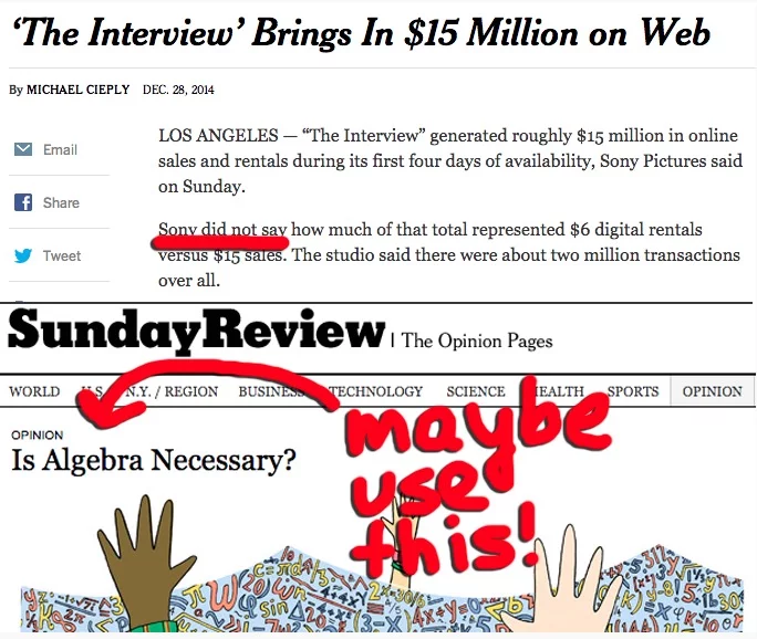
Over the holidays, the New York Times delivered an unusual juxtaposition of headlines and content, and apparent lack of self-awareness, to illicit such a hearty chuckle from its readers as to make the cheerful Old Saint jealous.
[image originally provided by @ddmeyer on Twitter.]
To those imbued with the skill of basic high school Algebra 1, the information in the article about Sony’s revenues for the first four days of release of “The Interview” were enough to solve a unit value problem. If we let R = the number of rentals, and S = the number of sales; then,
R + S = 2 million
$6*R + $15*S = $15 million
With a little quick symbolic manipulation, we see that S = 1/3 million in sales and R = 5/3 million in rentals. That exercise provided just enough mental stimulation and smug self-righteousness to prepare for the day’s sudoku and crossword puzzles. #smug #math
However, not too far into the sudoku puzzle we might realize that a deeper, more instructive problem exists here, a problem that actually permeates all of our daily lives. That problem is related to the precision of the information we have to deal with in planning exercises or, say, garnering market intelligence, etc. A second reading of the article reveals that the sales values, both the total transactions and the total value of them, were reported as approximations. In other words, if the sources at Sony followed some basic rules of rounding, the total number of transactions could range from 1.5 million to 2.4 million, and the total value might range from $14.5 million to $15.4 million. This might not seem like a problem at first consideration. After all, 2 million is in the middleish of its rounding range as is $15 million. Certainly the actual values determined by the simple algebra above point to a good enough approximate answer. Right? Right?
To see if this true, let’s reassign the formulas above in the following way.
R + S = T
$6*R + $15*S = V
where T = total transactions, and V = total value. Again, with some quick symbolic manipulation, we can get the exactly precise answers for R and T across a range of values for T and V.
S = 1/9 * V – 2/3 * T
R = T – S
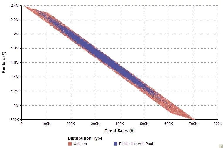
Doing this we now notice something quite at odds with our intuition – the range of variation between the sales and rentals can be quite large as we see in this scatter plot:
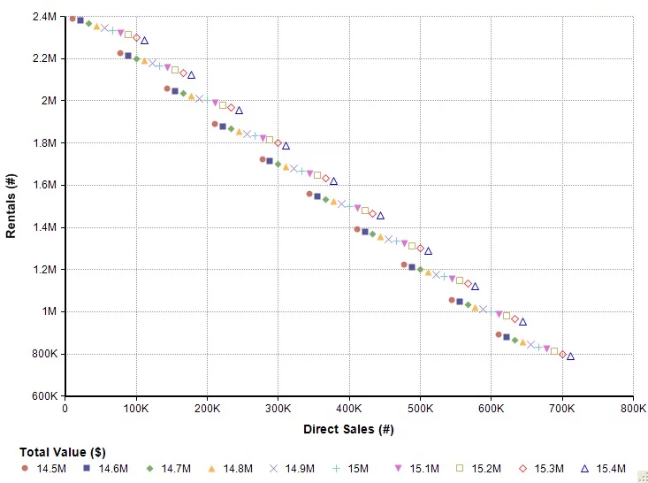
The distribution of total transaction values for various combinations of rental and direct sales numbers.
Here we see that the rental numbers could range from about 800 thousand to 2.4 million, while the direct sales could range from nearly 0 to 700 thousand! Maybe more instructive is to consider the range of the ratio of the rentals to direct sales:
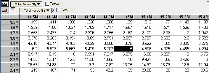
The distribution of the ratio of rentals to direct sales for various combinations of rental and direct sales numbers.
If we blithely assume that the reported values of sales were precise enough to support believing that the actual value of rentals and unit sales were close to our initial result, we could be astoundingly wrong. The range of this ratio could run from about 1.11 (for 1.5 million in total transactions; 15.4 million in sales) to 215 (for 2.4 million in total transactions; 14.5 million in sales). If we were trying to glean market intelligence from these numbers on which to base our own operational or marketing activities, we would face quite a conundrum. What’s the best estimate to use?
Fortunately, we can turn to probabilisitic reasoning to help us out. Let’s say we consult a subject matter expert (SME) who gives us a calibrated range and distribution for the sales assumptions such that the range of each distribution stays mostly within the rounding range we specify.
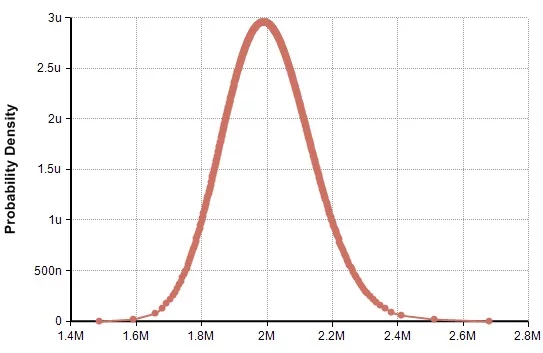
The hypothetical distribution of the total sales transactions assessed by our subject matter expert.
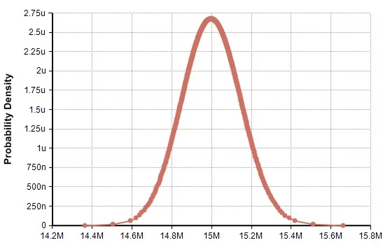
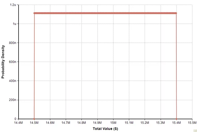
The hypothetical distribution of the value of the total transactions assessed by our subject matter expert.
Using the sample values underlying these distributions in our last set of formulas, we observe that in all likelihood – an 80th percentile likelihood – the actual ratio of the rentals to sales falls in a much narrower range – the range of 3 to 9, not 1.11 to 215.
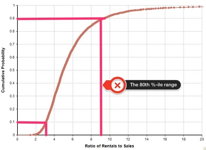
The 80th percentile prediction interval for the ratio of the rentals to sales falls in the range of 3 to 9.
Our manager may push back on this by saying that our expert doesn’t really have the credibility to use the distributions assessed above. She asks, “What if we stick with maximal uncertainty within the range?” In other words, what if, instead of assessing a central tendency around the reported values with declining tails on each side, we assume there is a uniform distribution along the range of sales values (i.e., each value is equally probable to all values in the range)?
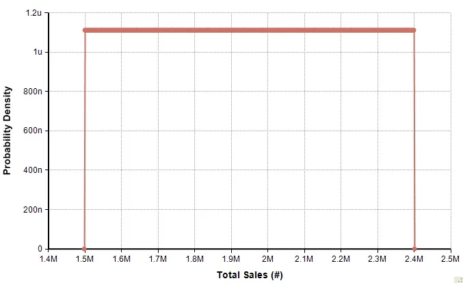
We replace our SME supplied distribution for total sales transactions with one that admits an insufficient reason to suspect that any value in our range is more likely than any other.
We replace our SME supplied distribution for total value with one that admits an insufficient reason to suspect that any value in our range is more likely than any other.
What is the result? Well, we see that even with the assumption of maximal uncertainty, while the most likely range expands by a factor of 2.7 (i.e., the range expanded from 3-9 to 1.7-18), it still remains within a manageable range as the extreme edge cases are ruled out, not as impossible but as fairly unlikely.
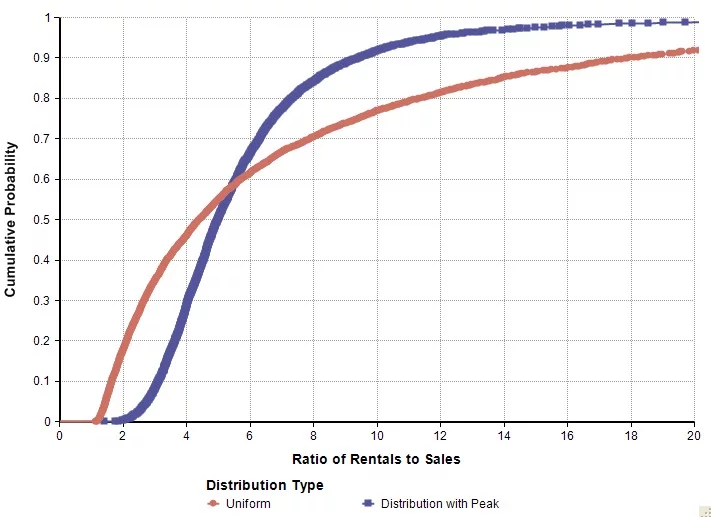
Replacing our original SME distributions that had peaks with uniform distributions flattens out the distribution of our ratio of rentals to sales, causing the 80th percentile prediction interval to widen. The new range runs from about 1.7 to 18.
The following graph displays the full range of sales and rental variation that is possible depending on our degrees of belief (as represented by our choice of distribution) about the range of total transactions and total value.
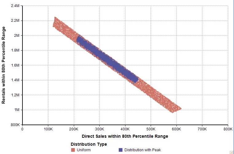
A scatter plot that demonstrates the distribution of direct sales and rental combinations as conditioned by our choice of distribution type.
By focusing on the 80th percentile range of outcomes in the ratio of rentals to sales, we can significantly improve the credible range to estimate the rentals and direct sales from the approximate information we were given.
A scatter plot that demonstrates the distribution of direct sales and rental combinations as conditioned by our choice of distribution type, constrained only to those values in the 80th percentile prediction interval.
Precise? Not within a hair’s breadth, no, but the degree of precision we obtain by employing probabilities (as opposed to relying on just a best guess with no understanding of the implications of the range of the assumptions) into our analysis improves by a factor of 13.1 (assuming maximum uncertainty) to 35.2 (trusting our SME). If our own planning depends on an understanding of this sales ratio, we can exercise more prudence in the effective allocation of the resources required to address it. Now, when our manager asks, “How do you know the actual values aren’t near the edge cases?”, we can respond by saying that we don’t know precisely, but using simple algebra combined with probabilities dictates that the actual values most likely are not.

