Analytica > Decision technologies > Monte Carlo simulation software

Monte Carlo simulation software: everything you need to know

What is Monte Carlo simulation?

Ready for some Monte Carlo? No, not a trip to the grand casino in Monaco — but rather a Monte Carlo simulation, a way to understand and manage risk and uncertainty using probabilities.

Quantitative models invariably rely on uncertain assumptions. Life and business unfold in unpredictable ways. Prices change, costs overrun, projects get delayed, the government makes new policies, natural and human-caused disasters happen, and there are breakthroughs in science and technology. How can decision-makers properly assess these risks and uncertainties and take their effects into account when selecting a decision strategy?

That’s where Monte Carlo simulation comes in. For each uncertain input assumption, you replace the conventional “best guess” with a probability distribution that expresses the uncertainty. The method selects a random value from each probability distribution and runs the simulation model to generate the results. It repeats the simulation hundreds or thousands of times to generate a random sample for each output of interest — the growth rate of a chain reaction, the return on investment, net present value, or whatever it is that you care about.

With a full distribution over possible futures, decision-makers can envision the full range of outcomes, and develop robust and resilient decisions to cope with them.

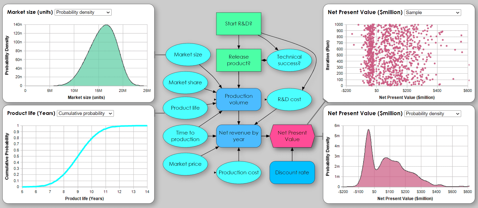
While Monte Carlo simulation originated in nuclear physics, it is now widely used by businesses and decision-makers of all types to analyze risk and uncertainty. Monte Carlo simulations are used to estimate and manage the uncertainty in return on investment, risks from pathogens or cyberattacks, to optimize inventory levels, plan product launches, and much more.

The mathematics underlying Monte Carlo methods may seem complex, but nowadays several software tools — like Analytica — handle all the complexities for you. They enable analysts and decision-makers to use these powerful techniques seamlessly and efficiently via intuitive use interfaces without requiring any special expertise.

Let’s dig deeper into Monte Carlo simulation to see why to use it, how to do it, and how using it effectively helps organizations thrive amid risk and uncertainty.

Why use Monte Carlo simulation software?

By far the most common, and the easiest, approach to uncertainty is to act like the proverbial ostrich, stick your head in the sand, and pretend that uncertainty does not exist. When building a quantitative model, wherever an input assumption is uncertain, you simply use what you think is the most likely or average value. This does not, however, guarantee that you will get the most likely or average value in the model results.

The “Flaw of Averages,” by Dr Sam Savage explains why this is a problem. The title refers to the common mistake that you can make reliable decisions by just using averages. But averages often hide important variations that can be catastrophic if you ignore them. Consider the man wading across a river with an average depth of 3 feet, as beautifully shown by this cartoon drawn by Danziger to illustrate Savage’s point.

The key advantage of Monte Carlo simulation is that it lets you explore uncertainties explicitly, understand the range of possible outcomes, and so avoid the often catastrophic effects of the “Flaw of Averages”. Monte Carlo simulation can provide a reliable inoculation against the natural biases, confusion, and, most importantly, wishful thinking that we often bring to dealing with uncertainty. Without Monte Carlo, you can make the decision that will be best only for a single “most likely” scenario, Monte Carlo lets you see how well each decision performs over the full range of possible futures. It helps you select a robust decision strategy that will work well over the entire range.

A quick history of Monte Carlo simulation

Let’s take a step back to the origins of the Monte Carlo method. It was invented by Stanislaw Ulam, a Polish-American mathematician and nuclear physicist working on nuclear fission at Los Alamos as part of the Manhattan Project. The idea first came to him when he was playing a card game in 1946:

“The first thoughts and attempts I made to practice [the Monte Carlo method] were suggested by a question that occurred to me in 1946 as I was convalescing from an illness and playing solitaires. The question was what are the chances that a solitaire laid out with 52 cards will come out successfully? After spending a lot of time trying to estimate them … I wondered whether a more practical method than “abstract thinking” might not be to lay it out [100] times and simply count the number of successful plays.”

In his research, Ulam was exploring the behavior of neutrons in the nuclear fission chain reaction. Ulam and his partner, John von Neumann, had a set of variables (e.g., velocity, time, direction of movement, path length, and type of collision) many of which were uncertain.

They then began experiments using early computer technology, assigning random values to as many as seven unknown variables to produce a probability distribution on the nuclear reactions of interest. Because the work was classified, it needed a code name. Ulam had an uncle that frequented the casino in Monte Carlo — the rest is history.

How to do Monte Carlo simulation

These are the key steps to perform a Monte Carlo simulation, given you have a computer model to forecast the effects of decision options:

Identify the input assumptions about which you have significant uncertainty. Elicit a probability distribution from a subject matter expert to express their uncertainty in each input. You might select a standard probability distribution, such as a uniform, beta, or normal distribution, or ask for 10th, 50th, and 90th percentiles and fit a distribution to them.
Fit probability distributions to data if you have relevant historical data on an uncertain input. Often you’ll need to adjust it to reflect future changes based on expert judgment, combining steps 1 and 2.
Generate a random sample of n values, typically 100 to 10,000, from each input probability distribution.
Propagate the uncertainty through the model by running it n times using the values from the random samples to generate a corresponding sample of values for each output variable.

View the uncertainty in key results as a probability distribution fitted by the software to each output sample.
Use sensitivity analysis to identify how much each input contributes to the uncertainty in the result or recommended decisions.
Choose a robust decision strategy that can be successful under a wide variety of possible scenarios.

It is usually a good idea to iterate this process. When sensitivity analysis identifies a few uncertain inputs that matter most to the result, you may redo step 1 and/or 2 to collect more expert judgment or relevant data to refine the input distributions.

In the next sections, we’ll explore these steps in more detail.

Where do you get the input probability distributions?

Would-be users of Monte Carlo simulation often wonder about how to obtain the probability distributions to express the uncertain inputs. The simplest approach is to consult a subject matter expert and ask them each to express their uncertainty by estimating the 10th, 50th (median), and 90th percentile of a probability distribution. You (or the software) can then fit a probability distribution to these percentiles. Or you can choose a standard parametric distribution that seems appropriate to represent the uncertainty, such as the Normal, uniform, triangular, beta, and so on, and estimate the parameters. Good Monte Carlo software should make it easy to select and fit a comprehensive range of distributions. There are widely used protocols to conduct this “expert elicitation” to help experts unfamiliar with subjective assessment of probability how to do this, and to minimize cognitive biases, especially the common tendency to overconfidence. If you consult more than one expert, there are simple ways to combine their assessments.

If you have access to historical data relevant to the quantity of interest, you can use that to guide the assessment. Say that you’re trying to estimate next year’s sales of a software product and have 10 years of past sales. You could estimate the mean and standard deviation and fit a normal distribution. Better yet, you could use time-series analysis to fit a trend line and estimate the uncertainty based on the quality of the fit to past data.

But, using the trend line assumes that future sales can be simply extrapolated from past sales, which involves a subjective judgment. More likely, you know things that won’t be visible in past sales data. Perhaps, your company is planning a big improvement in your product or a price drop, or you expect a major competitor to enter the market. There is no simple formula to adjust the forecast. Even when you have a lot of relevant historical data, you must still make a judgment that the future will be similar to the past if you want to simply follow the historical trend.

Sometimes people feel uncomfortable using “subjective” expert judgment when they are aiming at an “objective” analysis. But resorting to single “best estimates” and a deterministic analysis does not actually remove the subjectivity. A degree of judgment is unavoidable, since we can never get data from the future. It’s better to be explicit about it, and use a careful process to estimate and express the expert judgment and its associated uncertainties than to try to hide the inevitable judgments under the carpet of “fake certainty.”

Uncertainty: A Guide to Dealing with Uncertainty in Quantitative Risk and Policy Analysis, M. Granger Morgan and Max Henrion, Cambridge University Press: New York, 1990. ISBN 0-521-42744-4

How many samples do you need to run in a Monte Carlo simulation?

The number of samples used in Monte Carlo simulations typically ranges from hundreds to millions, depending on the required accuracy. A larger sample size yields more accurate estimates of the resulting distributions, including their mean (expected value), standard deviation, percentiles, and so on. But of course it takes longer to compute.

A common misconception is that the computational effort is combinatorial—i.e., it grows exponentially with the number of uncertain inputs. That would seem to make it intractable for models with many uncertainties. This is true for common probability tree (or decision tree) methods, where each uncertain quantity is divided into a small discrete number of outcomes. But, in fact, the great advantage of Monte Carlo is that the computational effort scales roughly linearly with the number of uncertain inputs—i.e., computation time is approximately proportional to the number of uncertain quantities. So it is usually quite practical for models with hundreds or even thousands of uncertain inputs.

The number of samples you need doesn’t depend on the degree of uncertainty or number of uncertain inputs in your model. Rather it depends on how much precision you want for the output distributions that you care about. Suppose you are interested in estimating percentiles of a cumulative distribution; there’s no need to increase the sample size just because you have more uncertain inputs. For most models, a few hundred up to a thousand runs are sufficient. You only need a larger sample if you want high precision in your resulting distributions, especially if you want a smooth-looking density function. Given the inherent uncertainty, higher precision needed for smooth density functions is usually an aesthetic preference rather than a functional requirement.

More efficient variants of Monte Carlo simulation

There are several techniques that can give greater precision for a given sample size than crude Monte Carlo sampling:

Latin hypercube sampling is the somewhat intimidating name of a widely used variant. For n samples, the distribution for each uncertain input is divided into n equiprobable intervals. For each sample, it selects one of those intervals (without replacement), and generates a random value from the interval. This method covers each input distribution more uniformly than simple Monte Carlo, and provides more accurate results, especially when the uncertainty in the result is dominated by just a few uncertain inputs.
Median Latin hypercube sampling is a variant of Latin hypercube that uses the median of each equiprobable interval instead of random sampling from it. This method (the default in Analytica) gives even more accurate results for a given sample size. To dig deeper into this topic and see some examples, read the blog on Latin hypercube vs Monte Carlo sampling by Lumina CTO, Dr. Lonnie Chrisman.
Sobol Sampling is a quasi-Monte Carlo method that tries to spread sample points out more evenly in probability space across multiple dimensions. It coordinates sampling across multiple dimensions, creating a more even sample than Latin hypercube, which spreads out sampling for each dimension independently. Sobol works well for simple models with up to around 7 uncertain quantities. But, unlike the other sampling methods, its convergence rate depends on the number of dimensions (uncertain inputs), so it is less effective for complex models with many uncertainties. For more see Sobol sampling in Analytica.

When you want to estimate a small probability of a catastrophic result—such as, the melt-down of a nuclear power plant, or extreme financial events that might lead to bankruptcy—standard Monte Carlo and related methods may converge slowly and so require huge sample sizes with millions of runs. In such cases, you want an accurate representation of the upper tail of a distribution, which might be only 1 percent probability or less.

Importance weighting can come to the rescue in such cases. It weights the sampling process to generate many more runs for extreme or catastrophic outcomes, and fewer runs that do not. At the end, it inverts the weights to remove bias from the distributions. This method can greatly improve accuracy in the tails of interest for a given sample size.
Sparse Monte Carlo simulation, developed by Sam Savage, is a related method for estimating low probabilities of disaster. It generates only samples with catastrophic outcomes, and so further improves simulation efficiency for low probability events. Here’s an example for managing the risks of explosions on natural gas pipelines.

How to view the results of a Monte Carlo simulation

The value of Monte Carlo simulation (like most quantitative analysis) is realized only when decision makers and other stakeholders understand the results. Clear visualization is critical. These are the most common ways to display the results of a Monte Carlo simulation as a probability distribution:

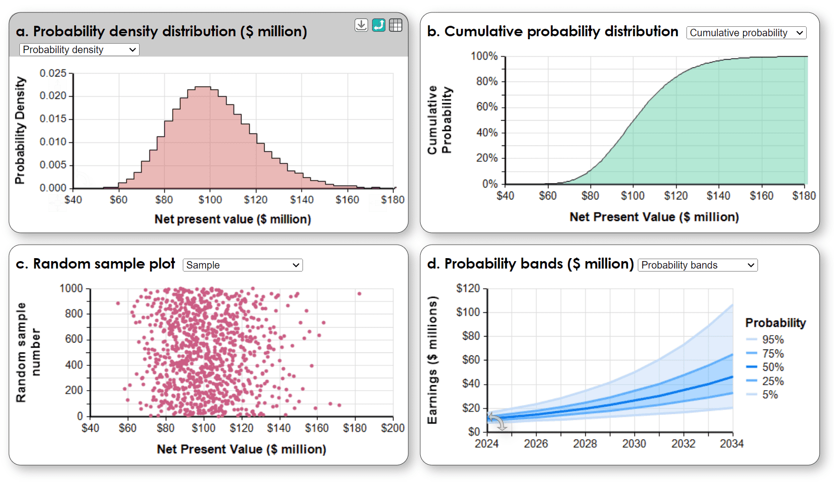
Histogram: Shows a frequency distribution of the simulation results for the Net Present Value of a project. The peak is the most likely value (mode) with variability below and above the mode. The vertical axis shows probability density or frequency. Most people have some familiarity with “bell-shaped curves”. They see that the height indicates which values are most likely, although most find it easier to understand as a frequency plot than a probability density function.
Sample plot: Shows all the points in a random sample generated by the Monte Carlo. The point cloud is a clear way to visualize a random sample and probability density, but is too much information for most people.
Cumulative Distribution: Shows the probability that the variable (Net Present Value) will be less than or equal each level. The median is the value ($100 million) that corresponds to the 50% cumulative probability. The cumulative is popular with risk and decision analysts, but less well understood by the general population.
Probability bands: Shows a series of distributions of earnings by year with lines indicating the percentiles (5%, 25%, 50%, 75%, 95%) for each point in time. These are a clear way to show a series of related probability distributions varying over time or another dimension.

Your choice of how to display probability distributions depends on your intended audience, what insights you want to communicate, and what decisions these displays should inform. It is sometimes useful to offer several views to emphasize different aspects of a distribution. Even better is an interactive display that lets users compare different views.

Sensitivity analysis: Which uncertainties matter?

Sensitivity analysis gives key insights into how much each uncertain assumption matters in terms of its contribution to the uncertainty in the results. These graphs illustrate four approaches to sensitivity analysis for a benefit-cost analysis of the decision on how much to control emissions from a power plant:

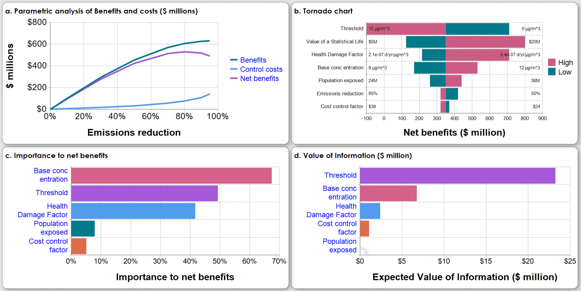
Parametric analysis shows how systematically varying an input parameter affects the results of interest. In this example, emissions reduction increases the expected net benefits (averaging over the distribution), the difference between benefits of saving lives (reduced mortality among people exposed to toxic emissions), and increasing Control costs.
The tornado chart shows the deterministic effect of varying each uncertain input from a low to high value (10th to 90th percentile of input distribution) on the net benefit, while holding all the other inputs at their median value. The variables are ordered by the range of effect from largest to smallest, giving a tornado effect.
Importance analysis compares the contribution of the uncertainty in each uncertain assumption on the uncertainty in the resulting net benefits. It uses rank-order correlation between the Monte Carlo sample for each input with the output. Each bar shows percent contribution with uncertain inputs ordered from largest to smallest importance.
Value of information analysis estimates the expected value of obtaining perfect information (finding out its true value) for each uncertain input on the improvement in expected value of the net benefit due to improving the decision on emissions reduction.

These four methods are useful in different situations. The parametric analysis visualizes the tradeoffs between lives saved and control costs. The other three methods offer ways to compare the relative effect of input uncertainties on the results. The tornado analysis can be deterministic or show expected values based on Monte Carlo simulation. It ignores interactions among the inputs in their effect on the results. The importance analysis averages the contributions of each input over the full distributions of all the uncertain inputs, and so does reflect interactive effects. The value of information is the most sophisticated method in that it estimates the value of obtaining full information about the actual value of each uncertain input in terms of improving the decision and hence improving the expected value of the outcome. It assumes that decision makers will actually select the decision that maximizes expected value. Its power comes at some computational cost, even using an efficient Monte Carlo method

Choosing Monte Carlo simulation software

Coding an efficient, reliable, and easy-to-use Monte Carlo simulation from scratch is a challenging software development project. Fortunately, there are several widely used software packages easily available that make Monte Carlo easy to apply. A good tool should include a comprehensive range of probability distributions; methods for handling correlated and dependent variables; fast and accurate sampling algorithms; tools to guide selection of sample size; a full range of ways to specify and view probability distributions and perform sensitivity analysis; and, ideally, integration with optimization tools to find robust decision strategies under uncertainty.

If your models are in an Excel spreadsheet, you can use a Monte Carlo add-in Monte Carlo package, such as @Risk from Lumivero, Analytic Solver from Frontline, and the SIPMath package. However, a retrofit add-in to Excel can have reliability issues.

It is often more convenient and reliable to use a comprehensive modeling environment, such as Analytica, which was designed from inception to treat uncertainty using Monte Carlo simulation. Analytica provides influence diagrams to structure and communicate models and probabilistic dependencies among variables, Intelligent Arrays to easily manage uncertainty over time, geographic regions, and other dimensions, powerful stochastic optimization, and an intuitive flow architecture for ease of modeling and transparency.

Author

Max Henrion, PhD, is the CEO of Lumina and creator of Analytica software. With a background in research, education, software design, and consulting, he has worked across energy, healthcare, aerospace, and more. A former professor at Carnegie Mellon, he also led decision technology teams at Ask Jeeves. Max received the 2014 Decision Analysis Practice Award and the 2018 Frank Ramsey Medal.