In a post on LinkedIn, David Vose argues that the advantages of Latin Hypercube sampling (LHS) over Monte Carlo are so minimal that “LHS does not deserve a place in modern simulation software.” [1] He makes some interesting points, yet products like Analytica and Crystal Ball still provide LHS and even offer it as their default method. Why? Are we, the makers of these simulation products naïve? As the lead architect of Analytica for two decades, I’ve explored this question in detail. I’ve compared the performance of LHS vs. Monte Carlo on hundreds of real-world models. And I’ve concluded that yes —it does make sense to keep Latin Hypercube as the default method.
Let me explain why I disagree with David Vose on some issues and agree with him on others. Several of his complaints are specific to Crystal Ball or @Risk and don’t apply to Analytica. Then I’ll add some key insights garnered from my own experience.
What is latin hypercube sampling?
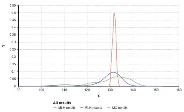
First some background. (Feel free to skip this if you already understand Monte Carlo and LHS.) Monte Carlo (MC) simulation generates a random sample of N points for each uncertain input variable of a model. It selects each point independently from the probability distribution for that input variable. It generates a sample of N values or scenarios for each result variable in the model using each of the of the corresponding N points for each uncertain input. From this random sample for each result, it estimates statistical measures such as mean, standard deviation, fractiles (quantiles) and probability density curves. Because it relies on pure randomness, it can be inefficient. You might end up with some points clustered closely, while other intervals within the space get no samples. Latin Hypercube sampling (LHS) aims to spread the sample points more evenly across all possible values [7]. It partitions each input distribution into N intervals of equal probability, and selects one sample from each interval. It shuffles the sample for each input so that there is no correlation between the inputs (unless you want a correlation). Analytica provides two variants: Median Latin Hypercube (MLHS) uses the median value of each equiprobable interval. Random Latin Hypercube (RLHS) selects a random point within each interval. The impact of LHS is visually evident in the following Probability Density Graphs (PDFs) that are each created using Analytica’s built-in Kernel Density Smoothing method for graphing, using samples generated from MC, RLHS and MLHS.

Convergence rate
MC and LHS are both unbiased estimation techniques: computed statistics approach their theoretical values as the sample size increases. You can make up for MC’s inefficiencies by increasing the sample size. But the real question is how many samples do you need to get to a given level of precision? Or conversely, at a given sample size, how much sampling error is there in the computed results? The concept of convergence rate addresses these questions. People also use the term variance reduction. Consider this example: I generated a sample of N=100 points from a standard Normal(0,1) distribution using each method and computed the sample mean. RLHS and MC each end up with a non-zero value as a result of randomness in sampling, where MLHS estimates the mean as exactly zero. I ran this sample of 100 points 10,000 times for each method and computed the standard deviation of the computed sample mean, as a measure of sampling error:
Here, the sampling error for MC is 20 times larger than for RLHS. Increasing sample size, the sampling error of 0.005 at a sample size of N=10,000—a one-hundred-fold increase in the number of samples. Published theoretical results for the univariate show that the sampling error of Monte Carlo goes down as O( 1/sqrt(N) ), [2], whereas the sampling error for LHS is O( 1/N ), quadratically faster, for almost all distributions and statistics in common use [3], [5], [7]. In other words, if you need N samples for a desired accuracy using LHS, you’ll need N2 samples for the same accuracy using MC.
Multivariate simulation
But this result holds only for the univariate case—when your model has a single uncertain input variable. When your model has multiple probabilistic inputs, the convergence rates for LHS start looking more like those for Monte Carlo. This happens because LHS shuffles each univariate sample so that the pairing of samples across inputs is random. With more variables, this randomness from shuffling becomes the dominant source of randomness. However, there is controversy about whether the improved convergence rate from LHS over MC is significant in real-life multivariate models. Numerous publications (e.g., [3], [4], [6]) show improved performance, where others found little practical improvement (e.g., [1], [8]). In my experience, LHS usually has a measurable advantage when there are up to three uncertain inputs with similar contributions to the uncertainty of the result. With more than three equally contributing inputs, MC and LHS are about the same. This is only a simplified guideline that doesn’t account for other relevant factors. For example, Manteufel [8] found the advantages of LHS to be less for highly non-linear models than for linear models.
David Vose illustrates that LHS has little advantage in his experiment summing nine equally distributed uncertain inputs. He finds that the difference between MC and LHS at a sample size of N=500 is insignificant. That’s consistent with my guideline that LHS has little advantage with more than three uncertain variables contribution comparable uncertainty. But, in many real-life models, even where there are dozens of uncertain inputs, we find that just a few uncertain inputs account for the lion’s share of the result uncertainty, so LHS still helps.
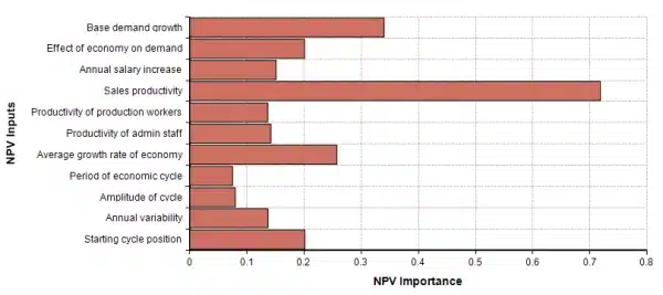
To illustrate this, I carried out an analogous experiment to Vose’s using a large corporate financial model with 41 uncertain inputs, but where a single input contributes the lion’s share of uncertainty to the computed expected net present value of future earnings. You can see this by using Analytica’s Make Importance feature on the result variable, shown here.
This Importance analysis plot shows the relative contribution of each uncertain input variable to the computed result. Several of the items show are array-valued inputs, so that in total there are actually 41 total uncertain inputs. One input in particular, Sales productivity, contributes far more to the net uncertainty than the others.
I ran the experiment 100 times for each of the three sampling methods, in each run recording the computed expected net present value, and then graphed the distribution of these computed results as show here.
The distribution of computed ENPV over 100 repeated simulations. Even with 41 uncertain inputs, the difference in performance between MC and LHS is still visible.
The standard deviation (a measure of sampling error) for each method is as follows:
This experiment illustrates that in a large real-world model, even with many uncertain inputs, it is still possible for LHS to substantially outperform MC in the common case where the a few uncertain inputs account for most of the result uncertainty.
Memory & speed
David Vose also argues that LHS has a downside of requiring more memory and computation time that MC. This is not true for Analytica, where both techniques take equal time and memory resources. I have personally invested a lot of time and research into optimizing the sampling algorithms used by Analytica to be state-of-the-art and have incorporated numerous optimizations to ensure that its LHS sampling is fast. For example, Vose argues that generating normal variates for LHS requires inverting the normal CDF function, which requires expensive numeric integration because there is no algebraic closed-form representation of the inverse CDF. But, Analytica uses a sophisticated and little-known, algorithm for CDF inversion for normal and related distributions that is about as fast as the best MC methods. It uses a two-stage rational polynomial approximation invented by Peter J. Acklam in 2003. As a result, Analytica has no significant speed differences between LHS and MC for the common distributions. If you are implementing your own simulation software, and don’t have the time to find or invent and implement such efficient algorithms, as David Vose points out, you can expect reasonable-to-implement algorithms for MC variate generation to run faster than the CDF inversions for LHS in your own custom software.
Where speed matters
Over the past 15 years, I have profiled hundreds of Analytica models to explore where they spend their computation time, and to look for speed-up opportunities, including eliminating any speed differences between LHS and MC. I recall none that spent a noticeable fraction of computation time on random sample generation. In pretty much all models, the bulk of the computation time is spent computing the model. So actually, if the sample generation method was a little slower than another, it wouldn’t really matter in practice.
Copula methods
David Vose writes “copula methods…would not be possible with LHS”. This is somewhere between misleading and untrue:
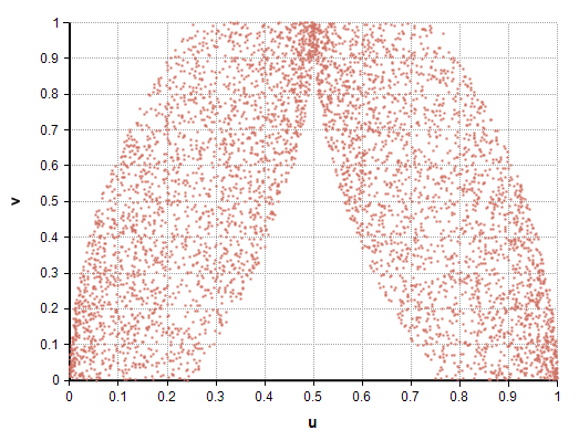
A 2-dimensional copula is a distribution P(u, v) over random variables u and v, each having a range of [0,1], and with marginal distributions, P(u) and P(v), as Uniform(0,1). Copulas can represent exotic correlation structures. Here’s an example of a 2-d copula structure.
A copula structure generated using RLHS.
If u and v are each sampled independently, any correlation is trivially impossible to capture since u and v are independent by construction. This is true whether you sample u and v using LHS or MC. I believe this is the reasoning behind Vose’s statement that such correlation structures are impossible to generate using LHS.
One approach to generating a copula structure is to transform a set of auxiliary random variables into the hypercube. You sample x1, x2, …, xm, and then compute a function u = u(x1, x2,…, xm) and v=v(x1, x2,…, xm) to produce the (u, v) copula. The auxiliary variables, xi, can be sampled just as well using MC or LHS. The copula graph above used RLHS on the variables v, x in the following:
v,x ~ Uniform(0,1)
u1 = If y<0.5 then y/2 + v/4 else 1/2 + y/2 – v/4
u := if u1<1/4 then 4*u1^2
else if u1<1/2 then 4*u1 – 4*u1^2 – 1/2
else if u1<3/4 then 4*u1^2 – 4*u1 + 3/2
else 8*u1 – 4*u1^2 – 3
This is an arbitrary copula that I put together for this article to illustrate a copula with a fairly arbitrary-looking shape. The theory behind how I derived it is beyond the scope of this article. The point is simply that LHS and MC are equally applicable to sample generation for copulas like this.
The better default
As I explained, MC has essentially no speed or memory advantage over LHS in Analytica. Theoretical results show that even in the multidimensional case, LHS methods converge faster than MC [3], [5]. In many cases, LHS outperforms MC substantially, even with many uncertain variables as we saw, due to the fact that a few uncertain inputs account for the lion’s share of the uncertainty in the result. Analytica’s built-in importance analysis can help you identify these cases. In other cases, where more than about three uncertain inputs contribute substantially to the uncertainty in the result, Vose is correct that LHS’s convergence advantages are minimal. The most compelling advantage of LHS, and MLHS in particular, is that it produces a clear depiction of each input distribution, devoid of sampling artifacts. Each input distribution looks smooth, even at the small sample sizes often used while developing and debugging a model. In sum, LHS (and MLHS) has important advantages over MC for some common purposes (viewing input distributions and computing models with a few variables dominating uncertainty in results), and no disadvantages in other situations (models with many contributing uncertainties and copulas): That’s why we will continue to offer it as the default in Analytica.
References
[1] David Vose (2014), The pros and cons of Latin Hypercube sampling, Linked In posting, 8 July 2014.
[2] Lumina Decision Systems, Analytica user guide, Appendix D: selecting the sample size.
[3] Christoph Aistleitner, Markus Hofer and Robert Tichy (2012) , A central limit theorem for Latin hypercube sampling with dependence and application to exotic basket option pricing, International Journal of Theoretical & Applied Finance 15(7).
[4] Mansour Keramat and Richard Kielbasa (1997), Latin Hypercube sampling Monte Carlo estimation of average quality index for integrated circuits, Analog Integrated Circuits and Signal Processing, 14(1/2):131-142.
[5] Wei-Liem Lom (1995), On the convergence rate to normality of Latin Hypercube Sampling U-statistics, Purdue University Tech Report #95-2.
[6] Jung Hwan Lee, Young-Don Ko and Ilgu Yun (2006), Comparison of Latin Hypercube Sampling and Simple Random sampling applied to Neural Network Modeling of HfO2 Thin Film Fabrication, Transactions on Electrical and Electronic Materials 7(4):210-214
[7] McKay, Beckman and Conover (old) — find paper. They had found empirically that univariate variance was greatly reduced by LHS. One of earliest LHS papers.
[8] Randall D. Manteufel (2000), Evaluating the convergence of Latin Hypercube Sampling, American Institute of Aeronautics and Astronautics, AIAA-2000-1636.


