This blog will be visiting the dart-throwing method of estimating π and comparing how fast or slow different sampling techniques converge to the actual value of π. The sampling techniques compared here include simple Monte Carlo (MC), Median Latin Hypercube (MLH), Random Latin Hypercube (RLH) and Sobol sampling — the four methods provided by Analytica.
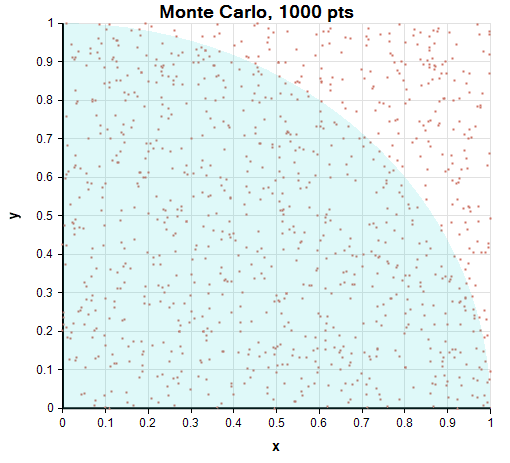
If you throw a dart at a square so that your darts hit randomly (i.e., uniformly) in the area of the square, on average π/4 of your dart throws will land inside a circumscribed circle. This is because the ratio of the area of the circle to the area of the square is π/4. Equivalently, you can throw darts at the first quadrant of a unit square with a circumscribed unit circle. This gives a simple (but not very efficient) way to approximate the value of π — just throw a lot of darts, and then multiply the fraction that land in the circle by 4, and this will give you an estimate of π. The more darts you throw, the more accurate your approximation will be. Here is what 1000 random throws into the first quadrant unit square looks like (using pure Monte Carlo):
One thing to notice about this scatter plot is that Monte Carlo’s coverage is spotty. For example, no darts landed near x=0.65 and y=0.55, while three darts landed at nearly the same location at x=0.23, y=0.89. This spotty coverage slows the rate that Monte Carlo converges to the correct value of π — more samples are required to obtain a given accuracy.
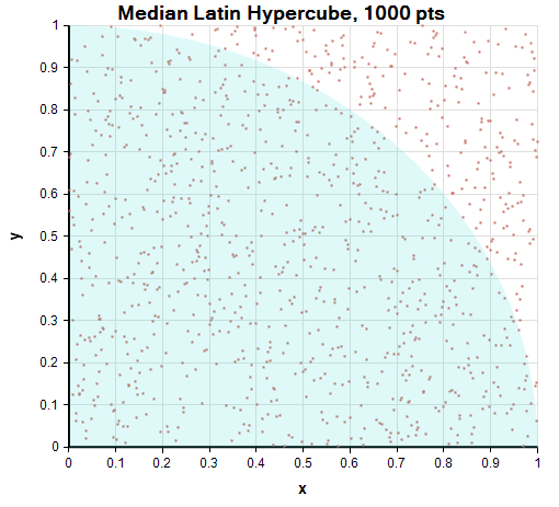
The other sampling methods were developed to improve on Monte Carlo’s convergence rate by spreading out the samples more uniformly. Median Latin Hypercube spaces the samples evenly along each axis, but then shuffles the x-coordinates and y-coordinates independently. As a result, the distance between any two points is guaranteed to always be greater than 1/sample Size = 1/1000 = 0.001. We’ll see below that MLH reduces the empty spaces and clustering meaningfully in a 2-D simulation, although it is hard to detect by looking at the scatter plot.
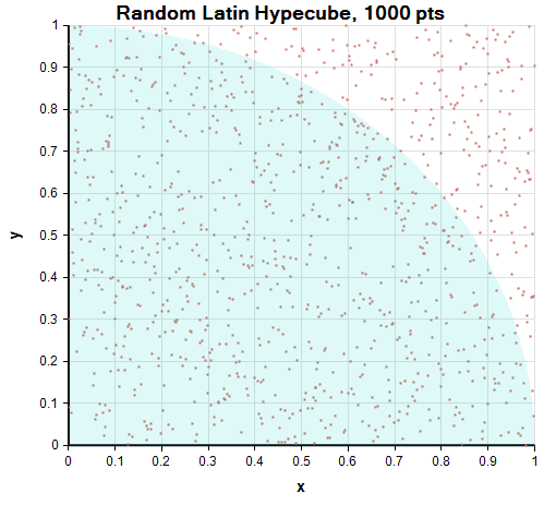
Random Latin Hypercube partitions each axis into equal intervals, and then randomly picks one point within each interval. As with MLH, it then shuffles the x-coordinates and y-coordinates independently. You can no longer guarantee that the distance between any two points is greater that 0.001, but the probability of that happening is still much less than with simple Monte Carlo. Once again, we’ll see below that this extra spreading helps in a 2-D simulation but is hard to see visually from the scatter plot.
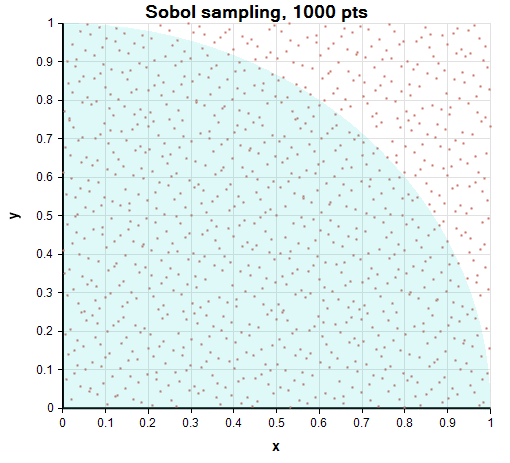
Finally, Sobol sampling coordinates the x and y coordinates so as to spread the points out as uniformly as possible in the 2-D space. The uniform spacing is much easier to see visually.
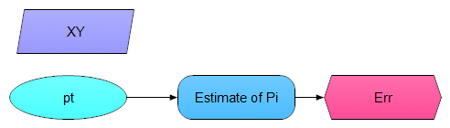
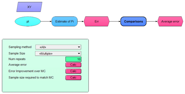
To simulate dart throws and compute π from them, I created a small Analytica model.
The dart-throwing plots above are the result plot for pt. The estimates for π from a single 1000-point simulation are:
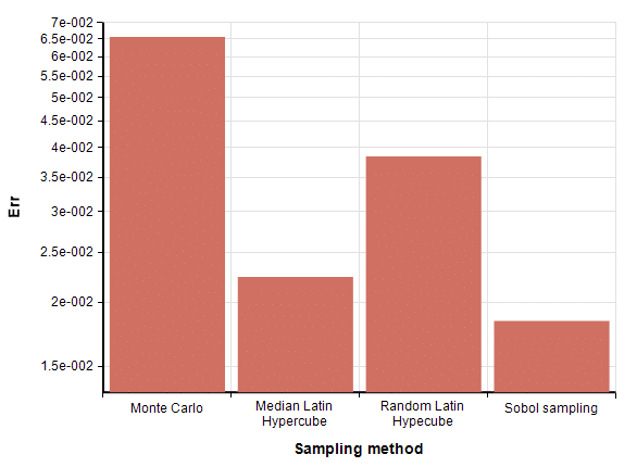
MC: 3.076 MLH: 3.164 RLH: 3.18 Sobol: 3.16
The difference between these and the true value of π are shown in this bar chart.
When you start over and do an entirely new run, the numbers change a bit each time. To smooth those fluctuations out a bit, I repeated the experiment 50 times and averaged the errors together. I did this by creating an index name Repeat and then changing pt to sample independently along that index.
Num_repeats := 50
Index Repeat := 1..Num_repeats
pt := Uniform(0,1,over:XY,Repeat)
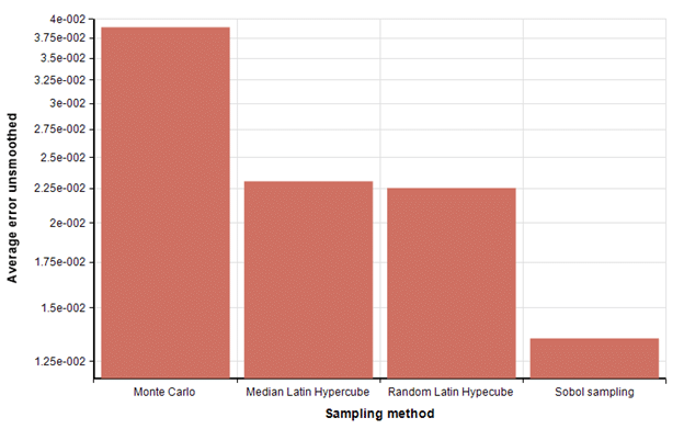
I then average Err using Mean(Err,Repeat). Now the average error is
So, from this we see that the two Latin Hypercube methods have similar performance on this problem with 1000 dart throws, both obtaining a 70% improvement in accuracy compared to MC. Sobol obtained a 180% improvement in accuracy over MC.
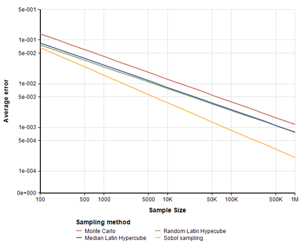
I expanded the model to loop over 17 different sample sizes log-spaced evenly between 100 and 1 million. At each sample size, I repeated the experiment 50 times and averaged the results. The error as a function of sample size came out as straight lines when plotted on a log-log plot, with some random fluctuation. To obtain nice looking plots, fit a line to the log-log plot. With these runs, we see how the error (between the estimate and true value of π) varies with sample size.
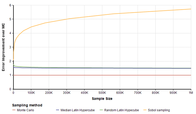
All three of the other sampling methods outperform MC by a substantial margin. To visualize this improvement better, I plotted the ratio of each curve above to the MC curve to see the multiple of improvement in precision compared to MC when using the same sample size.
Sobol obtains almost 6 times more precision at a sample size of 1 million. It is an interesting observation that the accuracy of Sobol gets better at larger sample sizes. This is consistent with theoretic results that predict its rate of convergence here should be O( {{(ln n)^2}over n}, where as MC’s theoretical rate of convergence is O(1 /sqrt(n)) .
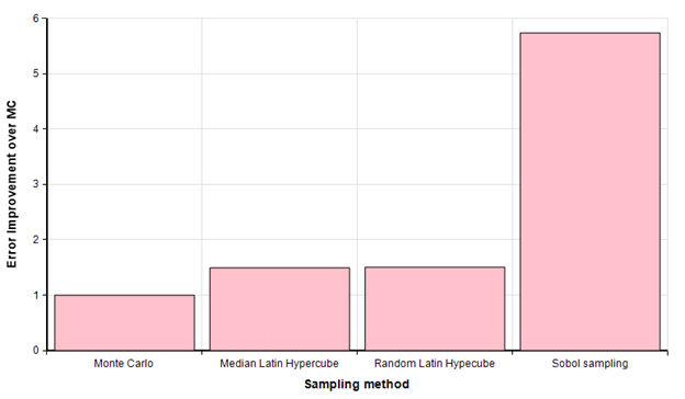
We can view the same result as a bar chart, here looking at the improvement in error at sample size of 1M.
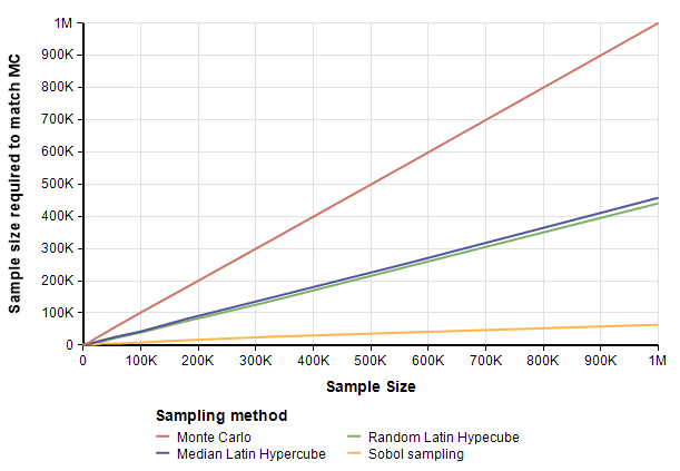
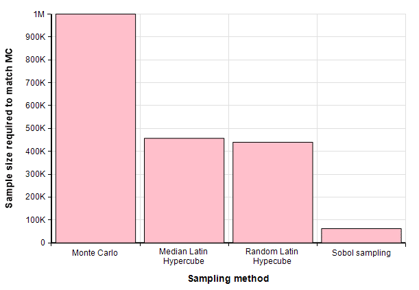
Another way to compare the sampling methods is to ask how many samples would each of the other methods need to match the precision of MC when MC is run at a given sample size.
Zeroing in on this same result when the Monte Carlo sample size is 1 million, we see that both LHS methods require about 440 thousand samples (a bit fewer that half) while Sobol reaches the same precision with only 50,000 samples. Hence, you ought to be able to achieve the same precision in about half the time with Latin Hypercube, and the same precision in about one 20th the time with Sobol sampling.
Today’s example had only two scalar uncertainties (x & y). Most real world models have many more uncertainties than this, and when there are a lot more uncertain quantities, all for sampling methods are much closer to each other. See an early blog article Latin Hypercube vs. Monte Carlo Sampling that discusses this in more detail.
The dart throwing approach is one of the most inefficient methods for computing π. However, it is both fun and educational to see it in action. If you’d like to play with these simulations, feel free to download my full model, which the code for repeating the runs across all sample sizes, sampling methods and number of repeats, with all the above visualizations of relative performance. To use, you can install the the Free Analytica edition, in which you’ll be able to run the sample sizes up to 32K. Analytica Developer or Optimizer users can run them up to as high as your computer’s memory and your patience allows.
Lonnie Chrisman is Lumina's Chief Technical Officer, where he heads engineering and development of Analytica. He has a PhD in Artificial Intelligence and Computer Science from Carnegie Mellon University and a Bachelor’s degree in Electrical Engineering from University of California at Berkeley.
Share now
See also
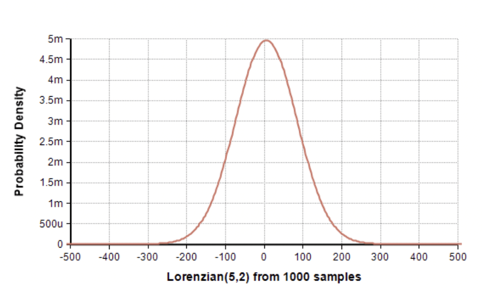
How the strange Cauchy distribution proved useful
On Tuesday I had an interesting exchange with Jorge Muro Arbulú, a professor in Peru, about the Cauchy distribution, which also called the Lorenzian distribution.
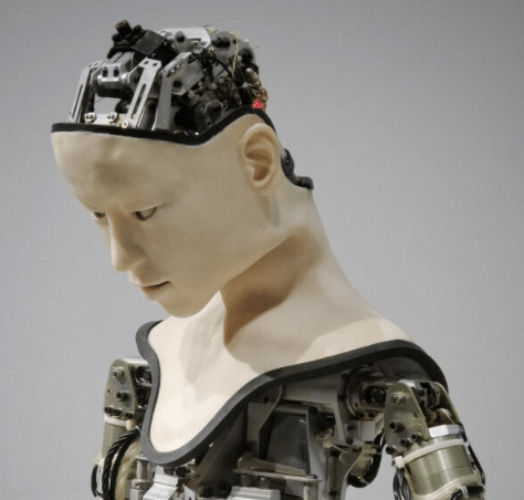
Could humans lose control over advanced AI?
Researchers used Analytica's influence diagrams to map out arguments and scenarios exploring risks with artificial intelligence (AI).
The value of knowing how little you know
Understand the Expected Value of Including Uncertainty (EVIU), compare with the Expected Value of Perfect Information (EVPI), and the insights it gives into a variety of problems.
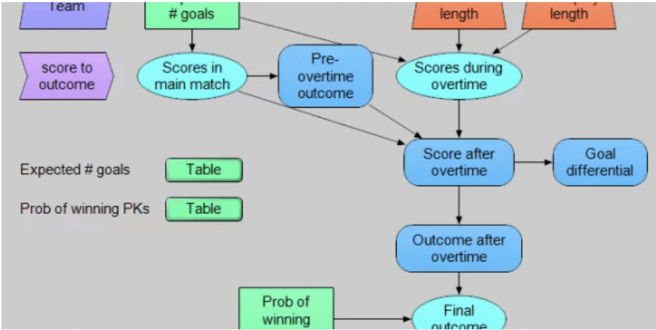
World Cup Soccer. How much does randomness determine the winner?
A few years ago France beat Croatia in the World Cup final. Congratulations to France for winning the last world championship! And also to Croatia for making it to the final...
Download Free Analytica
The free edition of Analytica includes these key Analytica features:
intuitive visual modeling with influence diagrams
the convenience and power of Intelligent Arrays
managing risk and uncertainty with fast Monte Carlo
sharing models on the web with the Analytica Cloud Platform (ACP)
Free Analytica has no time limit. The only constraint is it won’t let you create more than 100 variables or other objects. But your model can be quite substantial since each variable can be a multidimensional array. It also lets you explore, change inputs, and run existing models of any size (excluding features unique to the Enterprise or Optimizer editions).
You will need a computer using Windows OS to run Free Analytica.