This week, President Trump proposed new import tariffs on steel and aluminum. It seems as if the projected net impacts of these tariffs on the total US trade deficit and US economy depends largely on which news outlets you get your news from. We thought it would be helpful to put together a simple and easy to understand model to estimate of the net impact of these tariffs on the US trade deficit, assuming that no other factors change (e.g., no retaliatory tariffs are enacted by other countries). We wanted something that allows you to understand how its estimates are being derived, with assumptions that can be easily replaced with your own, so that the model itself would be impartial to any particular viewpoint. We want the uncertainties that are inherent in such a simple model to be explicit, so you can see the range of possibilities and not just a single guess. Finally, we wanted the model to be easy to understand fully for non-economists (a group to which we belong, too).
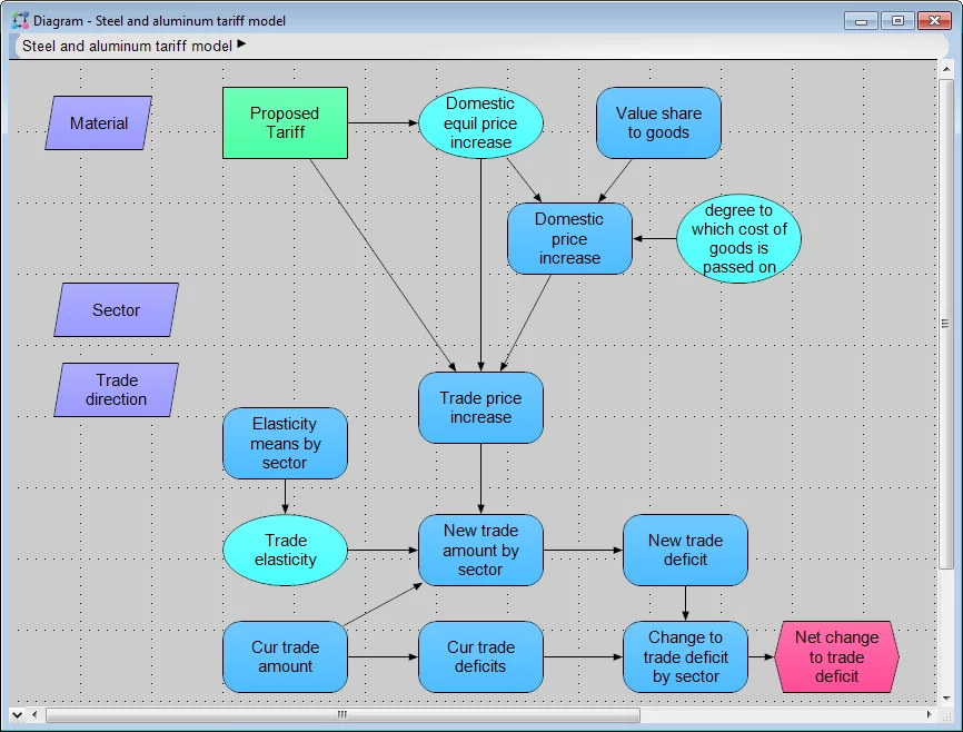
So here it is for you to explore and play with! You can interact with the model on the Analytica Cloud Platform (ACP) to change many of the basic assumptions, or if you want to enhance the model in more dramatic ways, you can install free edition of Analytica, download the model file to your own computer and improve away. We hope this type of exploration will help you to filter the plausible claims from the implausible, and maybe even to refine your own opinions!
Before we take too much criticism, we want to fess up to its many limitations. First, to keep it simple, we limited the scope of the analysis to just the US trade deficit. This is only one factor of many in the national debate. Second, a high quality economic model needs to model various equilibria (e.g., supply=demand) and numerous interactions and constraints. We intentionally avoided this level of economic complexity, since our primary goal is to have something that anyone with some quantitative skill and minimal economic background could grasp. Consider this common-sense level modeling, and not hard-core economic modeling – two steps up from working this out on the back of a napkin. Third, it is intentionally simple in excluding the rest of the world from consideration, so many relevant factors aren’t included. Especially important is the fact that we have NOT included any impact from trade wars that might ensue, although we will discuss below how you could incorporate your own ideas about this into the model if you are motivated to do so. And we have not incorporated any impacts due to currency fluctuations or economic weakening. Fourth, the model is populated initially with the best input data we could come up with with only a couple hours of effort. We readily plead guilty to all these simplifications. One criticism we hope we don’t hear is any claim that the model biased towards any particular position in this debate.
In the remainder of this blog posting, we’re going to tell you about the model, how it works, and what it forecasts based on our assumptions and the relevant data that we found.
What is an import tariff?
An import tariff on steel and aluminum is tax levied on steel or aluminum that in imported into the United States from another country. The tax is not levied on steel or aluminum refined in the United States. So, for example, if Acme Steel company in Canada sells Bob’s motor production company one trunkload of steel for $100, Bob would also need to pay the U.S. government $25 in taxes (for a 25% tariff rate on steel), bringing the cost to Bob up to $125. However, if Bob buys a $100 of steel from a US company, the tariff does not apply, thus giving the US company a competitive advantage.
With the new tariff, the rationally acting US steel company should raise its price to $124.99, since customer Bob would still prefer to buy their product than the $100 shipment from Canada. And hence, the tariff causes domestic prices for steel to increase. This margin increase for US steel company allows them to invest in more factories, hire more workers, and/or increase its profits, but, makes it more expensive for Bob to manufacture motors. As a result, Bob may need to raise his prices causing his US-built motors to be less competitive to motors built in other countries, making it harder for him to sell his product both in the US and abroad. Alternatively, Bob may decide not to pass his cost increases on to his customers to retaining his competitive pricing, by paying a price in terms of reduced profits (assuming he keeps his number of employees, and their salaries, the same).
In terms of trade deficits (the dollar amount imported into the US minus the dollar amount exported), we would expect the trade deficit for steel to decrease while the deficit for products made from steel would increase. The really difficult question is which effect is bigger? Even in the absence of trade wars, it is not at all obvious whether the import tariff would result in a net increase or a net decrease in the US trade deficit. And that is why it is useful to turn to quantitative models such as the one here.
President Trump’s proposal this week would impose a 25% tariff on steel imports from all countries, and a 10% tariff on Aluminum imports from all countries.
You may be surprised to learn that an import tariff on Steel is not something new for the US. The US imposed a tariff on steel imports as recently as 2002. After that tariff was rescinded, the US International Trade Commission analysed the impacts that the tariff likely had on several aspects of the US economy, which are contained in this report from 20031. This analysis is much more sophisticated than the one we present here, and may be of interest to those interested in how trade policy impact analysis can be done.
Our results
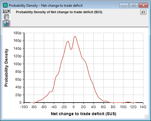
The result graph above depicts the net projected change to the US trade deficit, based on our simplistic model and our assumptions. The graph is a probability density graph, which shows the range of uncertainty in this prediction. The horizontal axis shows the projected annual change to the trade deficit as a result of the proposed tariffs (assuming no trade war ensues, etc.).
Two things were surprising to us: The almost perfect centering on zero (indicating that losses in the manufacturing sectors are essentially exactly equal to the gains in the steel and aluminum sectors), and the rather small range on the x-axis compared to the $19 trillion US GDP. Our model predicts a net change to trade deficit of less than $6 billion.
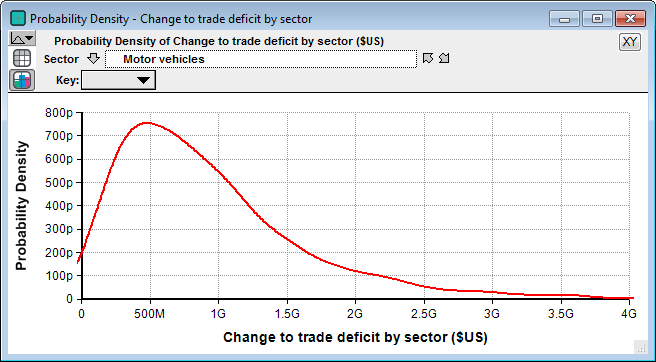
Among the industrial sectors as we have partitioned them, the sector with the largest projected trade deficit increase is the motor vehicles sector, with likely $500 million increase in trade deficit, but less that $3 billion.
We emphasize that this is a simplistic model, not good enough to be used for serious policy making, but that our goal is to obtain a model that is simple enough for even non-economists to fully understand. But by understanding this, it may help you to filter out the ridiculous from the plausible. For example, if you see someone claim that even if no trade war ensures, this tariff will increase our trade deficit by $50 billion, or conversely that this tariff will improve our trade deficit by $50 billion, you should question their credibility.
How our model works
The analysis basically consists of two steps. First, it estimates how much the price for something like a motor made in the US will increase as a result of the increased material cost, and then it estimates how that price increase (relative to motors produced outside the US) will alter the trade deficit.
Estimating price increases for steel and aluminum
With a 25% tariff, the cost of domestic steel in the US might increase as much as 25% (as reasoned above). However, eventually you can expect the actual cost of domestic steel to come to an equilibrium price that is less than a 25% increase, since the tariff incentivizes US companies to increase production capacity. Our simple model does not attempt to solve for that equilibrium, but rather allows you to estimate where it will be, which we have done with the expression
Triangular(0, 75%, 100%) * Proposed_Tariff
The first term, Triangular(0, 75%, 100%), is a probability distribution, which we are using to express our uncertainty in this estimate. It says the equilibrium price increase will be somewhere between zero and 100% of the proposed tariff, with a price increase at 75% of the tariff as the most likely value. Here is a great place to put in your own assumptions — if you think that no price increase in the most likely scenario, you can change the 75% to 0%, for example.
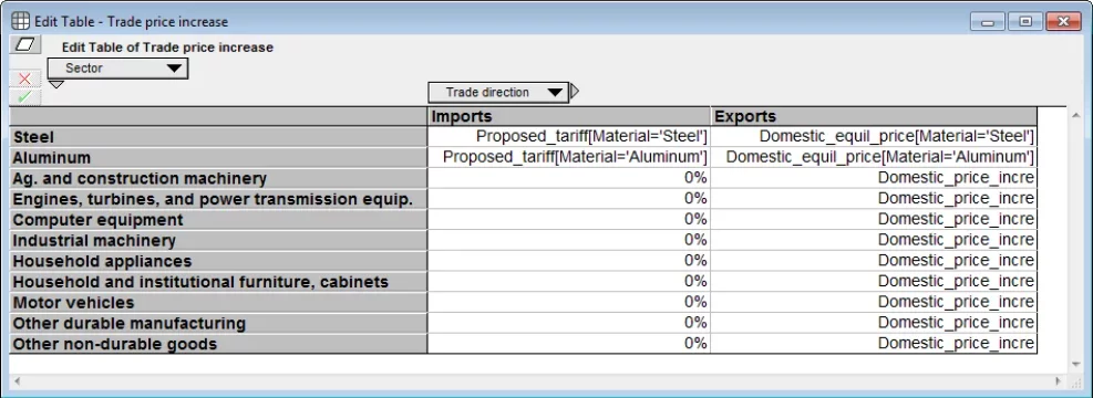
We reason that with no counter tariffs, the price at which US steel and aluminum companies export their product will equal the price for domestic customers. If you look at the edit table for the variable Trade_price_increase, you’ll see this encoded by the expression for Steel and Aluminum Exports, e.g.,
Domestic_equil_price[Material='Steel']
which says that the domestic equilibrium price for steel is to be used for the price that US exported steel is sold.
The price of steel from non-US sources will increase by 25% for US buyers. We’ve ignored secondary interactions that might force it to a new (lower) equilibrium. Since the US accounts for only 8% of global steel imports2, we felt this is reasonable. This is encoded in the Imports column for Steel (and similarly for Aluminum) in the variable Trade_price_increase as
Proposed_tariff[Material='Steel']
If you feel that market forces will push the international prices down by 10% once the US starts importing less, you can change this expression in that cell to
Proposed_tariff[Material='Steel'] * 90%
Estimating price increases for manufactured goods
The motor that Bob sells for $50 might contain $2 of steel. The other $48 is not directly impacted by the increase in steel price. We call the ratio of $2 to $50 the “value share to goods” of steel, which is a quantity specified in the model for each industrial sector in the variable with that name. We adapted numbers given in the US International Trade Commission’s 2003 report1 and sought aluminum data from the Bureau of Economic Analysis4 for our estimates of these values across a handful of economic sectors (e.g., motor vehicles).
The variable titled “degree to which cost of goods is passed on” is a number between 0 and 1 that encodes the degree to which US companies pass the cost increase in steel and aluminum on to their customers. A value of 0 means they absorb all cost increases (in reduced profits), a value of 1 means they pass it all on. Steel and aluminum are special cases here, which should be set to 1, but for every other sector we have used a probability distribution which considers are values between 0 and 1 as plausible, but with 0.5 being the most probable.
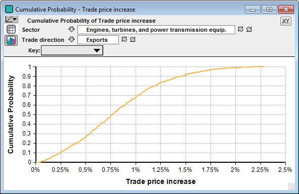
The variable “Percent price change” combines these, and then in Trade_price_increase the table uses this for the price change for US goods exported, but 0 for the price change of manufactured goods imported. Hence, the computed result for Trade_price_increase shows the impact on both import and export prices across sectors. The following result view show the Cumulative Probability graph for prices changes in the Engines, turbines and power transmission equipment sector.
Cumulative probability for the percent increase in export prices for engines, turbines and power transmission equipment. The vertical axis is the probability that the actual percent change in price is less than the value on the horizontal axis.
How prices alter trade deficits
Once Bob’s company increase the cost of a motor from $50 to $50.30, while non-US companies don’t increase prices on the international market, we expect there to be some decrease in sales. The sensitivity of sales to price increases is known as price elasticity. The price elasticity is a number, an elasticity of 2 means that a 1% change in price results in a 2% change in sales. In general, price elasticities might vary from sector to sector, and the import price elasticity may be different from the export price elasticity. We’ve provided our elasticity estimates based on a sector-by-sector analysis done by the group from Purdue University that put together the Global Trade Analysis Program (GTAP)3. For most sectors, the import elasticity is less than one. We were not able to quickly find sectoral estimates for export elasticity, so, we’ve left them as 1. Of course you can replace any of these elasticities with your own.
The key “magic” happens in the variable titled “New trade amount by sector”. We use “trade amount” to encompass both imports and exports, and the result of this variable is the projected amount of exports and imports in US$ of each industrial sector.
The steps from total exports and total imports by sector to the net change to trade deficit is straightforward.
Incorporating your own assumptions
You can access the model from your flash-enabled web browser by clicking here. This launches the model on the Analytica Cloud Player (ACP). Or from a Windows computer, you can run the model in Analytica Free 101 (download the model file). At first, you’ll probably want to just browse our assumptions and understand what it’s doing, perhaps changing a number here or there, and for that the ACP option is great. If you want to get carried away with enhancements to the parameters or the model structure itself, we recommend doing it in Free 101.
You should first consider how you would change particular estimates that we have provided to reflect your own opinions, or to explore what-if cases. For example, you can change the proposed tariffs to different rates to see how things change, or change the 75% equilibrium point in Domestic equil price increase, or change Degree to which cost of goods is passed on.
The price elasticities, encoded in Elasticity means by sector, are among the most challenging to estimate. There are numerous publications that attempt to estimate these elasticities. We obtained what seemed like credible export price elasticities by sector3, but ended up using a default mean elasticity assessment of 1 for the import price elasticities. We bet you can improve on this!
The Trade_price_increase table encodes several simplifying assumptions, and therefore provides a place where you can easily relax them. For example, the 0% entries under Imports means that we assume the tariffs on Steel and Aluminum don’t impact the price for imported goods in those sectors. If you think the changes in US exports might alter the supply/demand on the international market enough to alter the price equilibrium, you could insert you estimates here for the % change in import prices at the new equilibrium. The Exports column sets the change in export prices to be equal to the domestic price increase for all sectors. This edit table is where you can change that assumption.
Like many paying attention to this debate, we are broadly interested in the answer to “What would the impact be of tariff wars?”, though we haven’t tackled that question in this exercise. Any foreign tariffs would effectively alter export prices. Hence, a simple take would be to add the foreign tariff percent, so the cells in the Exports column would be, e.g.,
Domestic_price_incre + 25%
For a 25% tariff levied uniformly by all other countries on that sector.
Summary
Our goal has been to create and provide a model that is super simple and easy to fully understand, and easy for you to run with to alter and expand. This is in contrast to the goal of building the most credible and sophisticated macroeconomic equilibrium model. We focused on a single consideration, the impact of the proposed tariffs on to US trade deficit, and didn’t include many other important political, social and economic considerations that are relevant to the policy decision of whether to adopt this tariff. We wanted an explicit representation of uncertainty to make clear that there is a range of possibilities. And most of all, we hope that you will find this sort of objective, impartial modeling to be helpful when navigating the very diverse and questionable claims being offered in the highly biased commentary found in different news sources and internet channels.
We hope you enjoyed this. If you do explore this model, or even better, insert your own assumptions, please share any insights you have in the comments below!
References
- Steel: Monitoring Developments in the Domestic Industry (Investigation No. TA-204-9). Report prepared by the U.S. International Trades Commission. Sept. 2003.
- Steel Import Report: United States, Q3 2017, Global Steel Trade Monitor, US Department of Commerce, International Trade Administration, December 2017.
- M.P. Gallaway et al. (2003) North American Journal of Economics and Finance 14:49–68.
- 2007 Use Tables. U. S. Bureau of Economic Analysis Input-Output Accounts Data.
- The Global Steel industry by the numbers, CNN Money, March 2, 2018.

