In 2002, I developed a statistical framework for testing whether your data provides statistically significant support for the hypothesis that A causes B. I published only one conference paper with some colleagues on the idea before moving on to other things, but I’ve always felt the idea was pretty novel and interesting. In this blog posting, I’ll resurrect it and attempt to explain the core idea. The published paper was:
- Lonnie Chrisman, Pat Langley, Stephen Bay, Andrew Pohorille, “Incorporating biological knowledge into evaluation of causal regulatory hypotheses”, Pacific Symposium on Biocomputing (PSB), Kawaii, Hawaii, January 2003. (PDF)
Statistical methods vs causation
People in pretty much every empirical field of inquiry use statistical methods to show that the patterns in their data are real and not just due to randomness. Authors who publish scientific papers use these methods to say that their findings are “statistically significant”. The term means that the probability of the observed support would be low if the hypothesized phenomena isn’t actually there.
Scientific inquiry is most often focused on “causal hypotheses” — showing that A causes B. Hypotheses like:
- The burning of fossil fuels causes global warming.
- Warming global temperatures cause stronger hurricanes.
- Elevated insulin levels cause Alzheimer’s disease.
- Watching too much TV reduces a person’s IQ.
- Awarding low grades to students on homework assignments causes them to do poorly on tests.
- Low unemployment causes inflation.
But (classic) statistical methods, based only on observed data, do not establish that a data set provides statistically significant support for a causal claim. These methods tell you only whether your data supports an observation about a data metric (“statistic”), like a correlation, a difference in average, or difference in variation.
These statistical methods thus serve as only part of the puzzle. To make the jump from observation to causation, you have to resort to background knowledge (i.e., beliefs about other causes and effects) or to experimental design involving controlled intervention. As several of the examples above illustrate, controlled intervention is often not a viable option.
A framework for causal hypothesis testing
In 2003, I was working with Pat Langley and other colleagues at the Institute for the Study of Learning and Expertise (ISLE) on the Stanford campus, attempting to apply Bayesian network causal discovery algorithms to microbiological data, with the goal of developing new tools for identifying genetic regulatory pathways. Various technologies were able to measure levels of gene activity in a cell, and we reasoned that (perhaps) with the help of machine learning techniques, a correlation between the activities of gene A and gene B might enable these algorithms to discover that gene A regulates gene B. Except, of course, for the obvious pitfall that correlation does not imply causation. This was compounded further by the fact that these experiments often collected measurements on tens of thousands of genes, with a comparatively small number of actual replications, opening the doors very wide for spurious correlations.
These challenges led me to develop a mathematical foundation for testing whether a data set provides statistically significant support for the hypothesis that A causes B. The framework defines a p-value, which is the probability of seeing at least as much support for causation as is present in your data set if in fact no causal relationship exists. A p-value of 0.05 or less could be used as a threshold for “statistical significance” in the same way it is used in classic statistics.
How is this possible? My key idea was that background knowledge makes this possible. The reason observations give us confidence that a causal relationship exists is because we can explain how the causation might occur in terms of prior causal knowledge that we bring to the table. We formalized this idea mathematically. Given prior background knowledge K, a data set D, and a hypothesis about causation H, the p-value measures the probability that another data set D’ would support H to the same degree (or more) that D supports H, in the context of the background knowledge, K. The “in the context of K” part is the part that is different from classical statistics.
To derive this mathematical framework, we did something unusual — we combined a Bayesian framework with a classical statistical framework. It is through this hybrid that I was able to bring background knowledge to bear while addressing a question otherwise formulated in classical statistical terms.
Formulation
So now it gets a little mathematical. First, you have to start with some formal concept of a model of the world. I’ll use the letter M to denote one such model, but there are many many possible models out there, infinitely many. In some of those models, A causes B. In others, B causes A, and in others, there is no causal relationship. Some of those models contradict things that you are pretty certain are true, so you should consider each of those unlikely to be the correct model. Other models agree with established theories so should have a higher probability of being the correct model of the world. Let’s suppose that exactly one model can be considered to be the “correct” model. In a Bayesian spirit, P(M), your prior probability distribution over the space of all possible models, captures your prior background knowledge before you see any data.
When A causes B in a particular model M, then P(H|M) = 1, where H is the hypothesis that A causes B. When there is no causal relationship, which might include the case where B causes A but not vice versa, or A and B are related by a common cause where an intervention on A would not change B, then P(H|M)=0. I don’t posit anything in between — either A causes B or it doesn’t in any conceivable world model.
P(H) is your prior belief that H is true, and it is equal to
which is the same as summing P(M) over only the models where A causes B.
A data set D is a collection of measurements sampled from the world using a particular measurement protocol, which I’ll call the “experiment”. Once you assimilate the information from this data set, your belief about whether A causes B changes to the posterior distribution P(H|D). Using basic rules of probability, this posterior can be written as a function of our knowledge P(M) as follows
When the data D increases your belief in H, i.e., P(H|D) > P(H), it would be fair so say that the data appears to support the causal hypothesis. But if you had re-run the same data collection experiment again, you would have gotten a different set of measurements, D’, and because of this random fluctuation you might have concluded the opposite, that P(H|D’)<P(H). So the question of interest is whether the apparent support of the causal hypothesis is real or just a fluke of randomness of measurements and sampling?
The Causal p-Value
In short, the causal p-value is the probability that apparent support in the data for causation is just a fluke. Assume that A does not cause B, denoted ¬H. This assumption is called the “null hypothesis”. Conceptually, when you incorporate this assumption, you delete all models where A causes B from the space of possible models. Now suppose you were to re-run your measurements to get a new data set D’ ~ P(.|¬H). You could repeat this again and again, each time getting a different data set D’. The p-value is
In other words, you run your experiment over and over, sampling a different D’~P(.|¬H) each time, and computing P(H|D’) each time. The outer probability measures how often this appears to support H as strongly as your original dataset appeared to. In the equation, posterior(H|D’) is the same as P(H|D’), and prior(D|¬H) is the same as P(D|¬H). I just used those to emphasize the conditioning on data, and to differentiate if from the outer Pr[ ], which is over P(D’|¬H) distribution.
pv(H;D), the p-value, is very different from P(H) or P(H|D). All are values between 0 and 1, and all are probabilities. But they mean different things. The p-value, pv(H;D) is a measure of how strongly the data supports the causal hypothesis (with a lower value indicating greater support). P(H) and P(H|D) are your prior and posterior beliefs about whether the causal hypothesis is true.
Applying the framework
In our 2003 paper, we applied this framework to a cancer pathway in human cells, in which a kinase signal transduction cascade interacts to turn a variety of genes on or off.
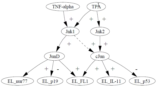
The first thing you have to do to apply this framework is define what your space of possible models looks like. Here is an example of a causal model from out work[1]:
In this model, extracellular stimuli (TNF-alpha and TPA) activate the kinase molecules Jnk1 and Jnk2. The five variables at the bottom denote the expression of five different genes. For example, the kinase molecule cJun suppresses the p53 gene. The + links (activation) and the – links (suppression) are examples of causal relationships. The arrow drawn with dashes is drawn that way to indicate a possible, but highly uncertain, causal relationship, and an opportunity to apply the framework to test whether a data set supports this causal hypothesis.
The full space of models consists of DAGs like the one shown above. Many arrows are possible between various stimuli, kinases and genes. After undertaking a fairly extensive literature search on these molecules and pathways, I assigned prior probabilities to each of these localized hypotheses, so that the prior for each model could be taken to be the product of the probabilities of the components assembled to produce the full model. Some pathways were pretty well established, and hence had high probabilities, whereas others like Jun1->cJun where quite open, and hence were assigned more entropy. In this manner, I was able to encode both the space of all possible models, and a prior measure P(M) over this space.
The calculation of the p-value required a lot of computational cycles. For that I used the Metropolis-Hastings algorithm, which is a Markov Chain Monte Carlo algorithm. This MCMC sampling was conducted over the space of all possible models, which was a very large and bumpy space, and getting the algorithm to mix adequately to arrive at a reliable computed result was the greatest challenge of the research. The Metropolis-Hastings algorithm is actually more of a sampling framework, enabling you to arrive at a specific algorithm by designing a proposal mechanism and distribution that specifies how the algorithm explores the space. Although I was creating the tool as a Java application, this part was so hard I ended up turning to Analytica and got the algorithm working there. I found Analytica so useful for this that shortly after this in 2003, I decided to re-join Lumina Decision Systems.
Subjectivity
The incorporation of prior belief into an evaluation of data will surely invite criticisms from some people that the analysis is not objective. By using your prior beliefs to interpret the data, are you prone to simply confirm what you already believe? Does this make you prone to find confirmation of non-existent effects?
Let’s consider the case of Alice and Bob, who have very different beliefs about the mechanisms that determine hurricane intensity. Their priors Pa(M) and Pb(M) are quite different, Alice is highly skeptical that an increase in global temperature causes in increase in average intensity, Pa(H)=0.1, whereas Bob is already pretty convinced it does, Pb(H)=0.9. They are presented with a data set D containing measurements of hurricane intensities with increasing intensities in recent years, along with increasing global average temperature measurements during the same time period. After processing the data, both might agree that the data D supports the causal connection between warming and intensity, so both might compute a similarly low p-value. However, Alice might still be a skeptic, e.g., Pa(H|D)=0.15 and Bob might be even more confident, Pb(H|D)=0.91. Note that it is possible that Alice finds the data more convincing that Bob, causing a greater shift from her prior to posterior, even though the data is less consistent with her beliefs both before and after.
So, subjectivity (a dependence on prior knowledge) does strongly influence the conclusions, but because the analysis is not asking the Bayesian question of whether hypothesis is true, but is instead asking the classical statistics question of whether the data supports the hypothesis, a confirmation bias that a stronger initial belief leads to a stronger conclusion does not necessarily follow.
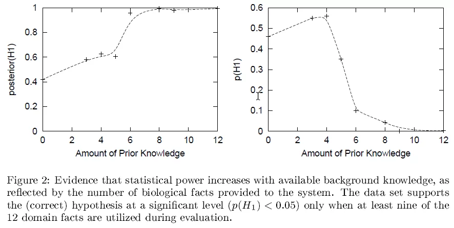
In the paper, we explored this a bit by carrying out experiments in which we varied the strength of the prior background knowledge, with the following results.
In these experiments, we found that when it started with more prior knowledge, it was more likely to be convinced by the data (larger P(H|D)) and was more able to detect statistically significant evidence for causation (pv(H;D)). This isn’t exploring the impact of blatantly false beliefs, just the accumulated amount of prior causal knowledge. I believe the improved ability to detect significance with increasing prior causal knowledge is a universal phenomena, but the impact on P(H) probably does not generalize universally.
Summary
Statistical methods are used to test whether patterns might be real or can be attributed to randomness. This enables you to identify reliable differences between groups and correlation between variables, but these methods alone don’t test whether a relationship is causal. In this post, I described an idea that my colleagues and I published in 2003 in a somewhat obscure conference, in which we developed a statistical framework for testing hypotheses about causality. The key insight is that learning a causal rule from observation is made possible by prior background knowledge about other causal relationships. We fleshed this out in a Bayesian-classical hybrid statistical framework which we were able to apply to a domain of gene regulation in human cells. Since moving on, I’ve always thought these ideas were pretty cool, but inadequately published beyond that one paper. I hope you enjoyed my resurrection and recounting of these ideas here.
If you enjoyed this, please remember to follow / befriend Lumina’s social media channels!


