Abstract: Bayesian linear regression made super easy and intuitive!

cost ≈ $2/mile * distance + $3
For any given ride, there will be a random fluctuation from the expected cost, so this is really just a model of the mean cost.
You had to come up with the parameters of this linear model — the $2/mile and the $3 fixed cost — based or your prior experience in other cities. Even though you are pretty experienced with these things, you’ll want to adjust parameters for this city as you get experience taking taxis here.
So now, you take your first ride in the new city, a 7 mile trip for $21. Your initial model predicts a cost of $17, so it seems like you should increase the two parameters of your model a bit. But by how much?
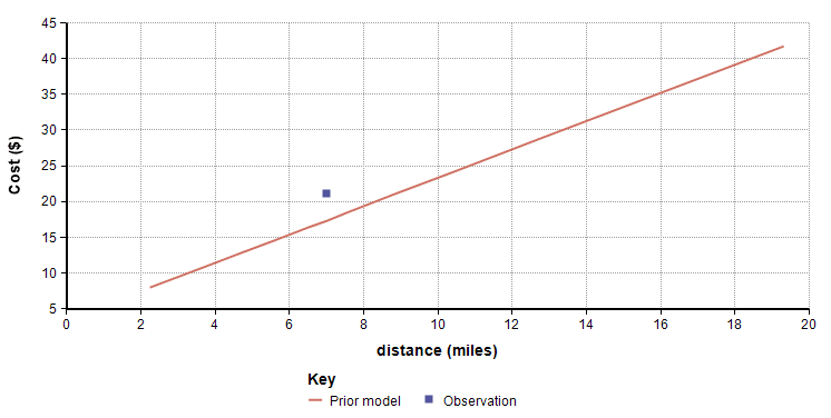
To answer this, you’ll need to also decide how “strong” your prior estimates are. To do that, I need you to estimate just one additional positive number, n, which represents the data-point equivalent information of your prior knowledge. n=10 could be interpreted equivalently in either of these ways
* Your prior is equivalent to information contained in 10 representative data points.
* With 10 new data points, your prior model and these new data points will contribute equally to your updated model.
When you estimate n, you’ll need to consider how extensive your prior experiences in other cities is, as well as how well you believe that experience will transfer to this new city. In what follows, I’ll use n=10.
The method for updating your model in light of this new data will be as follows:
- 1. Generate n representative values for distance: xi, i=1..n
- 2. Use your prior model to compute yi from these xi. These (xi, yi) pairs are called “surrogate data points”.
- 3. Add your newly observed datum to this set and fit a regression line through these n+1 points.
- 4. Use the slope and intercept from this regression for your updated model, and use n+1 for your prior strength parameter.
Step 1 of this method requires one additional item — a way of generating a list of representative distances of trips that you would actually take in this new city. It the language of statistics, this is saying that you have a probability distribution over the variable distance. In this presentation, this is not something that we update with additional data points. Here I’ll use a positive-only distribution with a 10-50-90 of 3 miles, 7 miles and 15 miles, which as an Analytica expression is UncertainLMH(3, 7, 15, lb:0). I like to use surrogate points that are equally spaced along distance quantiles, for example, with n=10 I use the 5%, 15%, 25%, …, 85%, 95% quantiles of distance.
The following graph shows 10 surrogate points from your starting (prior) model in red, along with the observed datum from your first trip in blue, and the best fit line to these 11 data points in green, which is the updated model after seeing one new data point.
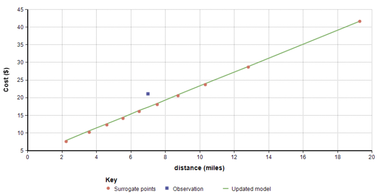
The updated model is now m=1.982, b=3.506 and n=11. Even though the model underestimated, the update actually decreased the cost per mile very slightly. Now you retain these three values as the representation of your new model, and don’t have to carry forward the actual data. After your take your second ride, just repeat the process by sampling 11 surrogates from the current model. Of course, if you happen to take several rides and forget to update, but you’ve retain those data, then you can also apply the procedure in one pass by adding the several data points in Step 3.
After the 10th taxi ride, the updated model becomes the green line in the following figure. I simulated the taxi rides and their mean costs using the model shown in blue with zero-mean noise added to get the cost data. The red line is the starting prior model.
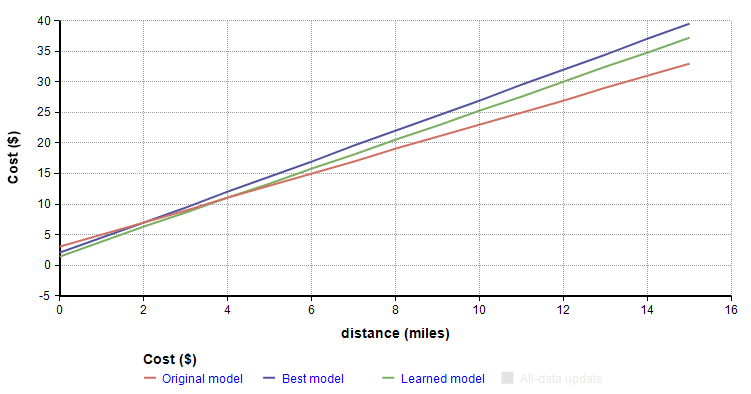
The updated model after the 10th taxi ride is m=2.378, b=1.492, n=20. At this point, the prior and observations should contribute equally, since we started at n=10. The slope started at $3/mile, whereas the blue line has a slope of $2.5/mile. The fixed-cost component started at $3 whereas the blue line has a y-intercept of $2.
Jump way ahead to the 90th taxi ride (for a 100-point equivalence of information) and it becomes hard to distinguish the learned model from the model used to simulate the data (the updated learned model, green, in mostly coincident with the blue “true” model):
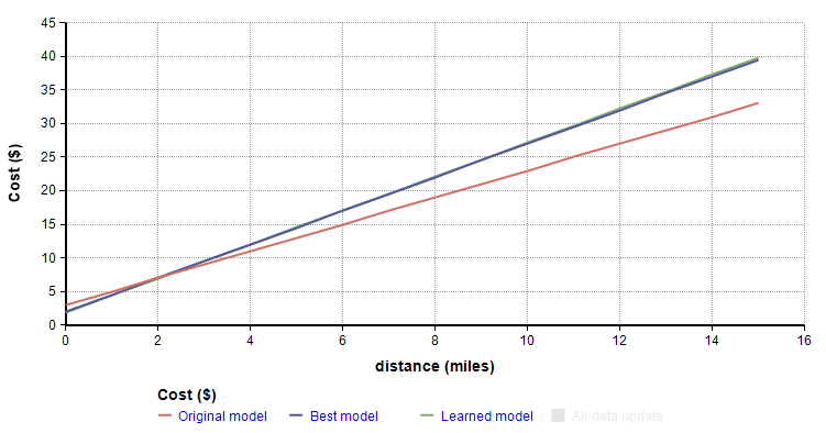
This update procedure is amazingly intuitive and simple. We treat our prior model as if it embodies the information of n data points, and we apply this by selecting n surrogate points to represent the prior, augmented by the observed data to enable a regression fit.
There is a literature in statistics on Bayesian regression, and Bayesian linear updating. The standard methods are quite complex and far less intuitive than what I’ve described here. They typically involve a description of a joint probability distribution over parameters b and m, as well as over σ2, the standard deviation of the noise. The trick with these is describing a conjugate prior distribution, where the word conjugatemeans that after updating, the posterior will belong to the same distributional family. Some exotic distributional families like the inverse-gamma, inverse-chi-squared, and multivariate Student’s t-distribution fill these roles, with parameters that are largely uninterpretable, thus complicating prior assessment and expert elicitation of parameters. Here, I haven’t employed any of these complex methods, which begs the question of whether the super simple process outlined here is consistent with Bayesian updating.
The surprising thing is that the simple and intuitive updating procedure described above is indeed consistent with Bayes’ rule! I have to credit Tom Keelin for this insight. He visited our Lumina office last week to give a presentation, and he convinced me of this. The mathematics behind this proof is far deeper and involved that I want to go into here. But the cool thing is that this could be a new and intuitive way to teach about Bayesian linear regression, and to provide a more pragmatically useful method for Bayesian linear updating, where the parameters that have to be assessed are interpretable.
The simple method reminds me a lot of Bayesian updating using a Dirichlet distribution. The Dirichlet is used to update a discrete probability distribution when a new outcome is observed. Suppose there are k possible outcomes. You start with prior probabilities for each outcome, in the form of k numbers between 0 and 1, that sum to 1, and you augment this knowledge with a number n, having precisely the same interpretation as the n used above, indicating that your probability vector has the same amount of information as n observations. After observing an outcome of i, your new pi becomes (n pi + 1)/(n+1), whereas the other probabilities become (n pk)/(n+1), and n is incremented by 1. Here n*pk is the effective number of times you’ve seen outcome k given your prior. Again, a very simple and intuitive update procedure and analogous to the linear model updating.
If you enjoyed this, please remember to follow / befriend Lumina’s social media channels!
