Marginal Abatement

Analytica models in the energy sector often include a Marginal Abatement graph for CO₂ emissions. In this post I explain briefly what a Marginal Abatement graph is and provide steps for creating one of these graphs in Analytica.

I have heard from numerous people that marginal abatement graphs are

insanely difficult to create in a spreadsheet environment, I’ve even heard some clients use the word “impossible”. As I’ll show, it is quite easy to produce a Marginal Abatement graph in Analytica.

What is a Marginal Abatement graph?

Google defines abatement as ” the ending, reduction, or lessening of something”.  Marginal in this context means “relating to or resulting from small or unit changes”. A marginal abatement cost is the cost required to reduce something by one more unit. A marginal abatement graph shows the marginal abatement cost as a function of the cumulative reduction.

When you want to reduce something, for example, total CO2 emissions, energy or water usage, or deaths from a disease, it is often the case that there are some actions that would be extremely cost effective, but can only do so much. We refer to these as the low-hanging fruit. Once we’ve taken those actions, the next possible actions will cost a little more per unit reduction, so that the more reduction we wish to achieve, the more it will cost per unit reduction.

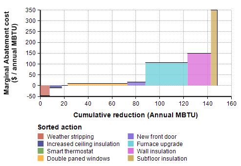
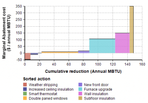
Suppose your goal is to reduce the amount of energy you use annually to heat your aging home. There are many actions you might take — upgrading to a more efficient furnace, replacing old weather-stripping, upgrading to double-paned windows, or having insulation injected into wall cavities. The following shows a hypothetical marginal abatement graph for such a situation.

Marginal abatement graph for home heating costs

The rectangles of different colors on the graph correspond to the possible actions, sorted left-to-right in order of cost effectiveness. On the X-axis we have the cumulative reduction. Weather stripping is cheap and easy, and in fact the most cost-effective, but will only save 8 MBTU/yr. Augmenting ceiling insulation is good for another 10 MBTU annually, so those together would achieve an 18 MBTU reduction.

The Y-axis reflects the cost incurred to save one additional annual MBTU. Weather stripping and ceiling insulation have negative costs, meaning that they more than pay for themselves, and the smart thermostat breaks even. The actions beyond those three incur a positive cost, so that you would need to justify those actions based on criteria other than costs alone.

When applied to CO2 reductions, the X-axis is usually cumulative annual CO2 emission reductions in units of tons CO2, the Y-axis is $ per annual ton CO2 reduction.

Starting information

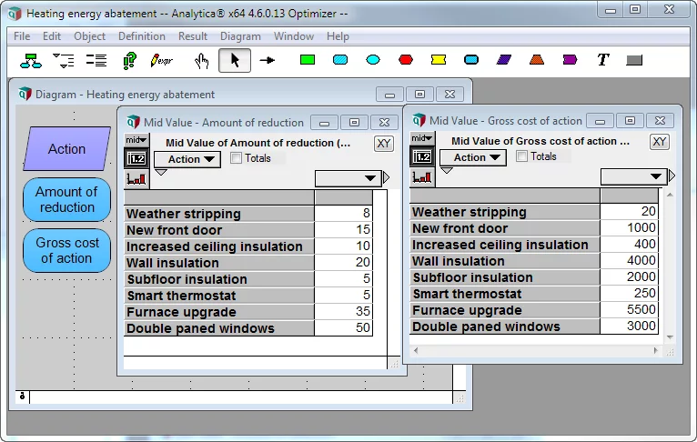
To start, you should have an index, Action, listing the possible actions available, a variable that computes “amount of reduction” that would be achieved from each action, and a variable computing “gross cost of action” for each action. In most models, each of these is an output calculation from a much larger model. How you come up with these is beyond the scope of this article.

Starting point for marginal abatement graph creation.

The amount of reduction is the annual reduction that will result from the indicated action. The gross cost of action is the one-time cost required to execute the action. In this heating example, these are all one-time actions.

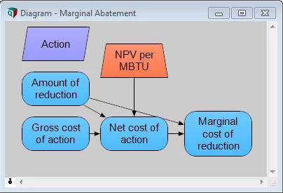
From these, you compute the net cost of action, which takes into account that there is a savings to be obtained from each action. In the current example, the savings is in annualized terms, but you will benefit from the annualized savings next year and the year after that as well. To combine the one-time costs with the annualized savings, you can express the cost of a unit of energy in terms of the net present value of one annualized MBTU saved. For example, assuming a discount rate of 10%, meaning that a dollar next year is worth 10% less than a dollar today, and $5 / MBTU, the net present value of a 1 MBTU savings would be about $50.  (Analytica expression: Index I := 0..30 do NPV(10%,$5,T)). The net cost of action is thus defined as:

Gross_cost_of_action - Amount_of_reduction * NPV_per_MBTU

and the marginal cost of reduction (Marginal_cost_of_red) is

Net_cost_of_action / Amount of reduction

Abatement model logic so far

Sorting and cumulating

The next step is to sort the actions, so that in the graph, the actions will be ordered from most cost-effective on the left to least cost-effective on the right.

Index Sorted_action := SortIndex( Marginal_cost_of_red)

Then compute the cumulated energy reduction over the sorted actions.

Variable Cum_reduction :=

Cumulate( Amount_of_reduction[Action=Sorted_action], Sorted_Action)

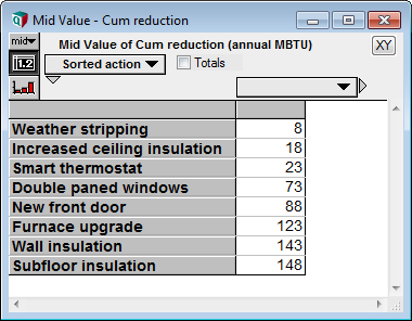
The main thing to notice here is that Amount_of_reduction has been re-indexed to Sorted_action, so that the cumulate occurs in the order of the sorted actions rather than in terms of the original (arbitrary) order of action. Here is the result — notice it is indexed by Sorted_action.

Cumulative MBTU reduction

The graph variables

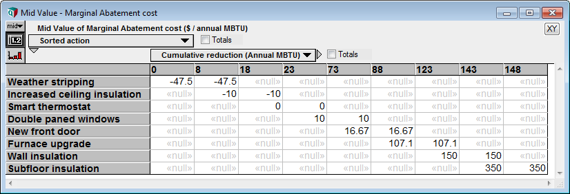
The “trick” to creating the marginal abatement graph is that we want a separate curve for each action, where each curve has its own color and its own key item. Each curve only has two data points — the left point and the right point, both at the same Y-value.  The plot is rendered as a filled line chart. To do this, you transform the data into the following form:

The form that the data for the abatement graph takes.

This is a 2-D array, so we need two indexes — Sorted_action and a new one. Cumulative_reduction. The Cumulative_reduction index has the values from the Cum_reduction variable above, with a zero prepended.

Index Cumulative_reduction :=

Concat( 0, CopyIndex( Cum_reduction) )

You can transform the data so that two data points land on each row, with the left point being at the level where the action has not been executed yet, and the right point being at the cumulative reduction after executing the action, as follows.

Objective Marginal_abatement_cost :=

If @Cumulative_reduction=@Sorted_action+1 or @Cumulative_reduction=@Sorted_action
Then Marginal_cost_of_red[Action=Sorted_action]
Else null

The @ operator in Analytica means “at the position”, so that @Cumulative_reduction returns the position of each element in that index. Hence, the expression @Cumulative_reduction=@Sorted_action means “on the diagonal”. The expression @Cumulative_reduction=@Sorted_action+1 identifies one cell off the diagonal where Cumulative_reduction is one larger (in position) that Sorted_action.

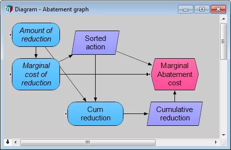
To keep your influence diagrams small, you can put the nodes used to produce the abatement graph in their own module. I like to use aliases for the main values before sorting, so it shows how they fit into the logic, and in this case, to turn on arrows to indexes.

The logic used to produce the marginal abatement diagram.

Finally, in graph view, pivot so that Cumulative reduction is on the X-axis, Sorted_action is the key. Double click to get to Graph Setup and select Line-only line style and Area Fill. You have yourself a marginal abatement graph — you might say it was as easy as weatherstripping.

Marginal abatement graph for home heating costs