In my earlier blog article, on marginal abatement, I explained what a Marginal Abatement graph is and how to set up such a graph in Analytica. In this article, I’m going to generalize that model to array-abstract over additional dimensions, and lead through the steps of setting up a graph handles the extra dimension(s). For me, this is an opportunity to illustrate issues and techniques that come up more generally in many modeling situation in which you want to make your model array-abstractable.
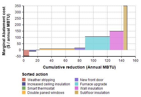
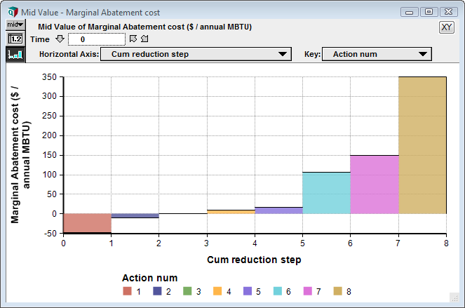
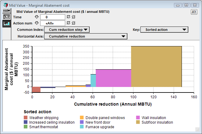
The above graph shows a marginal abatement graph for actions you have available for reducing your home heating costs. From the graph, we see that Weather stripping is the most cost effective upgrade, with the negative cost on the y-axis revealing that it more than pays for itself, but it is only good for up to 8 MBTUs per year. The next most cost effective upgrade is increased ceiling insultation, which also more than pays for itself and saves another 10 annual MBTU. The first Marginal Abatement blog post explains this in depth, so please read that article first.
Suppose that you have a partial reduction or marginal abatement cost for each action that varies along another index. These might vary over time, or you might introduce an index while conducting parametric analysis to examine sensitivity to input assumptions. The model from the first article does not handle the introduction of additional indexes for two reasons:
- Actions are sorted by cost-effectiveness, with the most cost-effective on the left, least cost-effective on the right. Once the data varies along another index, there is no longer a single sort-order. To generalize, we need to decide what to do about this.
- An index is used for Cumulative reduction, which is assigned to the horizontal axis of the graph. The numbers required for the horizontal axis varies along the extra index(es), so it is no longer possible to capture these in a single list. Said another way, in Analytica, and index must be defined as a single list — the extra index turns this into a multi-dimensional array, so it is no longer a valid index definition.
If you find that your own model does not array-abstract — i.e., it gets errors when you try to introduce a new dimension — it is likely that your problem is that you have a computed index, which depends on quantities that now have this extra index. If you don’t understand the issue, you should read the article Writing array-abstractable definitions. After that, you may get ideas for how to restructure things from the example here.
Data varying by time
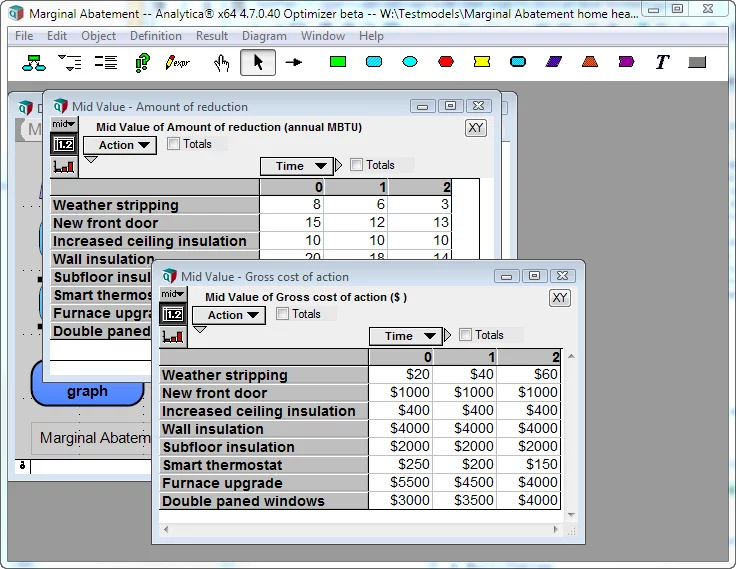
I start by adding a Time dimension to the two key inputs to the abatement graph, changing the cost of action and potential reduction per action so that they vary by time.
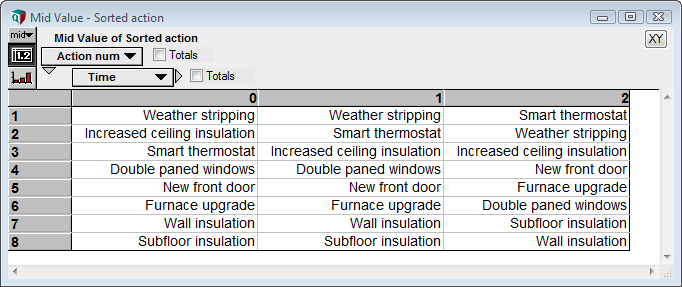
With this change, an error results when you try to view the result of Marginal Abatement cost. The error complains that the definition for Sorted_action is not a list. This happens because there is no longer a unique sort order.
Sort order that varies
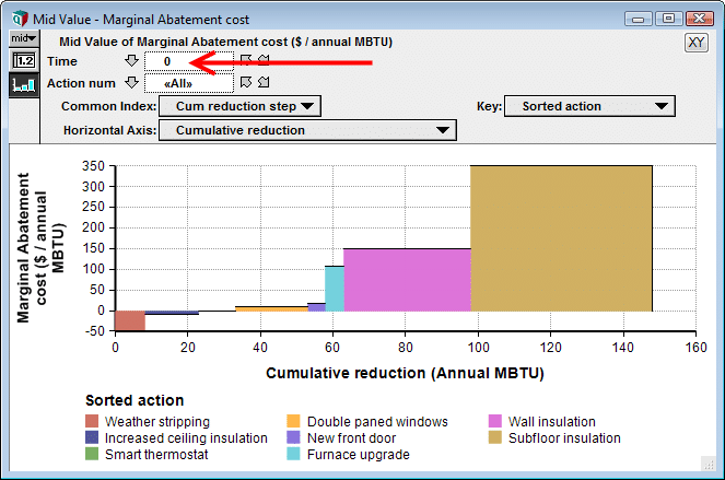
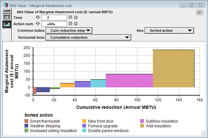
With an extra Time index, you have multiple marginal abatement curves, one for each Time period. Each abatement curve will, in general, have a different sort ordering of actions. I don’t think it makes any sense to overlay several abatement curves on the same plot, because that would be too crowded to see effectively. So what I’ll aim for is setting up the graph with the extra index(es) as a slicer, where Time appears in the following example.
As you increment the Time slicer, the graph changes. Each graph has a different ordering of actions.
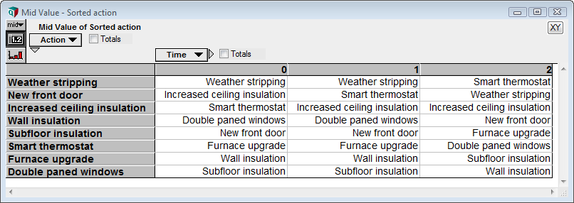
The Sorted_action index was defined as SortIndex(Marginal_cost_or_red). This breaks because now has two indexes — Time and Action — so it is ambiguous which index you are sorting over, and the result would not be a single list in either case. So the first change I’ll make is to change this node from an Index class to a Variable class, and to change the definition to
SortIndex( Marginal_cost_of_red, Action )This breaks the ambiguity — we are sorting over Action — and returns a 2-D array with a different sort order for each time period.
While this is now usable, I find the use of the Action index confusing for this array, since it is using the same labels. So I created a new index named Action_Num and defined it as CopyIndex(@Action), which is just the numbers 1 to 8. Then I reindexed by changing the Definition of Sorted_action to
SortIndex( Marginal_cost_or_red, Action ) [ @Action = Action_num ]
Cumulative reduction index
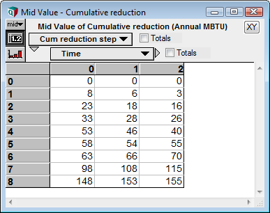
The next problem is that an index is used for Cumulative reduction. This was conventient for graphing, using the index for the x-axis, but once again, there is no longer a single list of cumulative reductions, but rather a separate list of values for each time step, so the result as it was written in the original model cannot be used to define the index.
I fix this problem in the identical manner that I fixed the sort order issue. I created a new index node, Cum_reduction_step, defined as 0..size(Action_num), then changed Cumulative_reduction from an index to a variable class. Previously, the definition of Cumulative_reduction has been Concat(0,CopyIndex(Cum_reduction)), which I changed to
Concat(0,Cum_reduction,,action,Cum_reduction_step)
This also prepends a 0 onto the original collection of Cum_reduction, but the fourth parameter, action, breaks an ambiguity about which index to prepend to, and the final parameter says to use the new index that I just created. Hence, we’ve collected the cumulative reductions separately for each time step.
The general technique for generalizing an index
Both problems above were addressed in the same way, which highlights a general technique that you may need to employ in your own modeling situations. You have a computed index, which returns a list until you introduce a new dimenion to your model Since the result is no longer a list, it is unable to array-abstract. The techique I used was to:
- Create a new index, usually with the elements 1..n, that will be replace your index variable as the index for this dimension. Its labels are now essentially meaningless, whereas your original index labels consisted of labels or values that were meaningful.
- Change the class of what had been your index into a Variable, and modify the logic to an expression that array-abstracts over extra indexes. This variable becomes a 2-D array (or 3-D when you add two new upstream indexes). The cells of this array now hold the meaningful values, which vary across the new indexes.
Creating the graph
The definition for the Marginal Abatement Cost result, the variable holding the final graph, used the two indexes that I just changed above. After substituting the newly created indexes for these in a straightforward way, the definition is now.
if Cum_reduction_step+1=Action_num or Cum_reduction_step=Action_num
then Marginal_cost_of_red[Action=Sorted_action] else null
The result graph is now
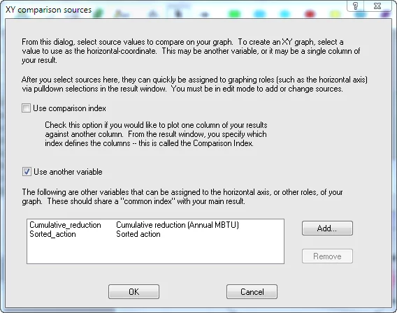
The x-axis and key are showing the index values, but not the values we want. We want to use the values from Cumulative_reduction for the x-axis, and the values from Sorted_action as the key labels. I call these value dimensions in the context of graphing, as contrasted to index dimensions. By using a value dimension, you can control what labels appear in each position. Initially these don’t appear as options on the drop downs for Horizontal axis or Key. To make them options, you need to first add them as Comparison Variables for the graph. Press the [XY] button and add them.
Finally pivot the graph roles and slicers to match those seen here.
Now it is possible to increment the Time slicer to view the different abatement graph, with different action order, for Time=1 or Time=2.
Summary
There are two interesting ideas demonstrated by this extension, both of which are applicable to situations having nothing to do with abatement. The first is the technique for structuring your variables and indexes so they array-abstract. The technique applies to the case where in a single situation you compute a list, which logically seems like it should be an index, but in which the computed values vary when new indexes are introduced to upstream variables. The second technique is the use of a value dimension for graph axis or key labels. If you aren’t already with the second technique, you may think you need your quantity to be an index so that you can use it for axis or graph labels, but in fact that is not the case.
I have seen marginal abatement graphs used in several real-world projects, and the extra index problem did not arise in any of those projects. Hence, the odds are that the simple instructions from the first marginal abatement article will work fine if you are interested in is creating an abatement graph.

