It’s tax week here in the US, and like many other people, I have less than a week to finalize my tax returns. I also have some last minute decisions. Should I, or my wife, put money into a traditional IRA or Roth IRA account? Should I continue contributions to my 401(k) account? Or should I be putting more of those savings into my standard “for-retirement” brokerage account? What is the best way to save for retirement, and which of these options will yield the greatest financial benefit for me by the time I reach retirement age?
To evaluate these options, I built a model that compares retirement plan options. The model looks only at financial return. There are many other factors that may be important to deciding which plan to use that I don’t consider, including differences in contribution limits, eligibility, funds or stocks that you are able to buy from the account, preferences for which financial companies you prefer do business with, how the account is treated when your kids apply for college financial aid, protections in the event you are sued, and whether the account is subject to probate after you die. For myself, I was also interested in comparing the performance of the tax-advantaged plans to a normal brokerage account. You might find the inability to access a 401(k) or IRA before retirement without a penalty to be an additional advantage (or disadvantage) over a brokerage account.
In this posting I talk about how to use the model, if you want to analyze your own situation, as well as how I went about modeling this, which may interest you if you are working on your own model building skills. I also used this as an opportunity to use some new Analytica 5.1 features to try something new and experimental — an interactive sensitivity panel contained within in a table.
Retirement account types
I consider four retirement account types: A standard brokerage account, a Roth IRA, traditional IRA and 401(k).
Brokerage account: This is just a standard account with no special tax treatment. You “contribute” post-tax funds, meaning that you’ve already paid income tax on the money you deposit, which you use to purchase stocks. Dividends are taxed in the year you receive them. Capital gains on stocks are taxed in the year you sell them. If you buy a stock and hold in until retirement, you capital gains taxes aren’t due until the end. When you reach retirement, you don’t have to pay any income tax when you withdraw your model. You may have capital gains to pay as you cache in your investments, but only on the profits.
Roth IRA: Like a brokerage account, you contribute post-tax funds to a Roth. But that’s the end of taxation. From then on, dividends and capital gains earned between now and retirement are not taxed, and no tax is due when you withdraw your money at retirement.
Traditional IRA: In a traditional IRA, you deposit pre-tax wages, which means you are effectively able to deposit more up front. Dividends and capital gains accrue and compound until retirement. When you withdraw your money at retirement, you must pay income tax on the whole amount withdrawn. Importantly, this is your income tax rate in retirement, whereas in a Roth, funds were taxed at your income tax rate today.
401(k): A 401(k) is an employer-sponsored plan that in terms of the financial parameters is essentially the same as a traditional IRA. As with the traditional IRA, you deposit pre-tax wages, then pay income tax when funds are withdrawn at retirement. The main financial differences between a 401(k) and traditional IRA is that you are allowed to contribute a larger amount each year to a 401(k), some employers match your contributions, and annual maintenance fees charged by your 401(k) bank tend to be higher on average for 401(k) accounts.
Income tax
Perhaps the most obvious differences between the account types is the income tax you have to pay, especially if you think your income tax rate in retirement will be different from your income tax rate today. In a standard brokerage account or a Roth IRA, you pay income tax at your current income tax rate. In a traditional IRA or 401(k), you will have to pay at your future income rate in retirement.
I asked several people whether they thought their income tax rate would be higher or lower in retirement. It seemed pretty clear for the people in their 20s that it would be higher, since a few were in school, and the others were just starting their career and considered their salary today to be lower today it would be later. After thinking about it a while, several others reasoned that it would be about the same as today. They would have a comparable standard of living, with taxable income sources from retirement accounts, pensions and social security. One person felt that because he would no longer be receiving taxable wages from working, it would be less. And one person was certain that tax rates would increase dramatically by the time he reached retirement, an inevitability due to the reckless deficits the government is running today. So there is no single correct answer here.
To understand how your income tax rates now and at retirement impact the return in a retirement account, it is useful to write out the equation for each case, which is easy to do under the simplifying assumption of a constant market rate of return, m, each year. For a Roth, the net value at retirement, xt, with retirement t years in the future, an initial investment of x0, annual account fees at a rate of f and a current income tax rate of r0 is
xt = x0 ( 1 – r0 ) ( 1 + m – f )t
In this equation, the starting investment amount is x0 ( 1 – r0 ). This then appreciates by ( 1 + m – f ), compounding annually. For a traditional IRA or 401(k), the net value is
xt = x0 ( 1 + m – f )t ( 1 – rt )
where rt is your income tax rate in retirement. In this case, your starting amount is x0. The ( 1 – rt ) term reflects the fact that you have to pay income tax when you withdraw your money. When r0 = rt, these are the same, implying that there is no difference in the rate of return between a Roth and traditional IRA or 401(k) if their annual maintenance fees are the same. When r0>rt, the traditional IRA beats Roth, and when r0<rt the Roth beats the traditional.
One counter argument is that even when r0 = rt, a Roth is still better because you can effectively contribute more. If you are under 50, you can contribute up to $5,500, which for a Roth means that x0 ( 1 – r0 ) < 5500, but for a traditional IRA you are limited to x0 < 5500. But even so, the rate of return is equal. (Note: The limit on the amount you are allowed to contribute phases out as your income level increases).
The simplified equations above use the assumption that the market rate of return is constant from year to year, which is clearly not true. If it fluctuates, the ( 1 + m + f )t term becomes Product( 1 + mt + f, t ) in both equations, and since both are impacted equivalently, the same conclusions about the effect of income tax rates still holds.
The compounding effect
My core interest with this modeling project was to compare the performance of a standard brokerage account to my 401(k). It is more difficult to write down a simple equation for the performance of a standard brokerage account, which will be subject to taxes on dividends, plus short-term and long-term capital gains taxes in the intervening years between now and retirement. This motivated me to build a model.
In a brokerage account, the taxes you pay on dividends and capital gains in the intervening years has an impact on your overall value by retirement. On the one hand, you’ll have to pay taxes on your profits sooner or later, but if you pay the taxes sooner, you lose out because you no longer earn the compounded return on those funds. So the frequency of trades is an important factor when predicting the performance of a brokerage account. If you frequently trade stocks, or frequently do major portfolio rebalancing, the increased trading turnover can cut into your gains from compounding. If you hold an investment without selling all the way to retirement, you get the full benefit of compounding. In an IRA or 401(k) account, because these intervening taxes don’t occur, you benefit from the compounding effect whether you trade often or not. Also, a stock with a high dividend rate cuts into your eventual value in a brokerage account since you need to pay taxes on the dividends.
Let’s look at the math behind the compounding effect. Suppose you have an investment value of x0 today, and we’ll compare two scenarios: (1) You hold x0 until retirement at time t, here upon you sell and pay your long-term capital gains tax, and (2) you sell today, pay g in long-term capital gains tax this year, and reinvest the remainder (at the same rate of return, m). Rewrite the today’s investment value as x0 = x’0 + g, where g is the capital gains tax paid and x’0 the amount reinvested in the second scenario. Let rg be the long-term capital gains tax rate (the subscript now is not time, but just part of the name). If we don’t sell, at time t the investment value grows to
xt = x0 (1+m)t = x’0 ( 1 + m )t + g ( 1 + m )t
whereas if we sell and pay the capital gains tax now, the net investment value is only xt = x’0 ( 1 + m )t. The difference is g ( 1 + m )t, which is all profit (gain). The final capital gains tax due on the x0(1+m)t part is the same in both scenarios, so the bottom line is that you end up with
difference = g ( 1 + m )t ( 1 – rg )
more by holding (not selling) until retirement. With a m=10% annual market return, rg=15%, and a t=15 years until retirement, you ultimately make $3.55 on ever dollar you pay today in tax. It pays off to avoid intermediate taxes.
The model
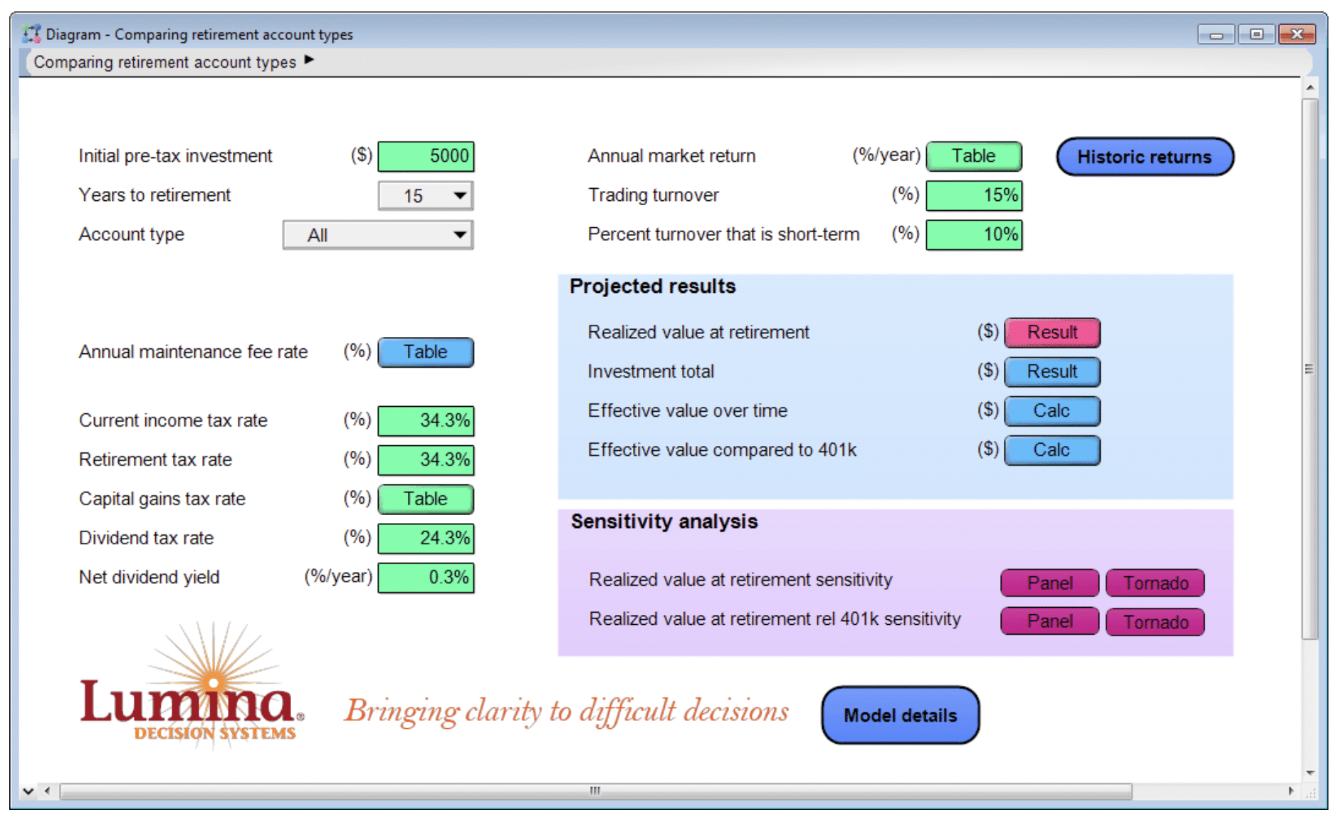
The model UI is shown here, where you can see the various inputs and results.
To try out the model with your own assumptions, you have two options:
- Install the free edition (if you don’t already have Analytica installed), then download the model and open it in Analytica.
You can also download a version of the model without sensitivity analysis, which has fewer than 101 objects and can hence be modified using the free edition.
For the full sensitivity analysis functionality discussed below, you should use the desktop Analytica application.
The above screenshot depicts the input parameters that characterize your personal situation, investment style and assumptions. These vary from person to person.
The model is designed to compare financial performance among different retirement account types for a one-time contribution. The contribution amount is a pre-tax amount, so the Traditional IRA and 401(k) accounts start out with the full amount, whereas Roth IRA and brokerage account types start out with less, whatever is left after income tax is paid.
When entering tax rates, keep in mind that these should be the sum of your state and federal rates. The 34.3% rate in the screenshot reflects a 25% federal and 9.3% California income tax rates. To estimate your future retirement tax rate, you may need to think a bit about your larger retirement plan. Are you planning to maintain your standard of living into retirement. Will you be drawing primarily off of social security and your 401(k) or IRA accounts, which are taxable income. If so, your current tax rate might be reflective of your retirement tax rate. (Note: Since this model is designed to evaluate only a one-time contribution. it doesn’t attempt to model the influence your account type choice has on your future tax bracket). Or, do you expect your taxable income sources to drop off in retirement, making your tax bracket much lower.
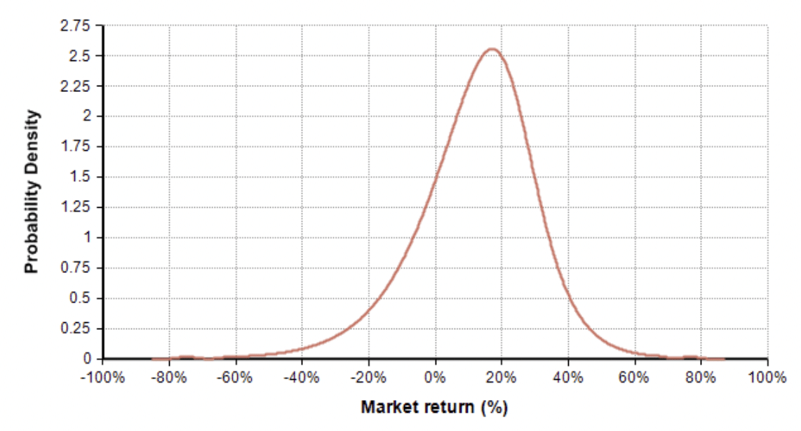
For capital gains rates, at the federal level, the short-term capital gains rate (for investments held less than one year) is generally the same as your income tax rate, whereas for most people the long-term rate is 15%. In California, the capital gain rates are the same as income tax rates, which is 9.3% for most middle-class earners. Dividend rates are also 15% and 9.3% (= 24.3%) for federal and California respectively. The annual market return is modeled as a probability distribution specified by a low-medium-high estimate (the 10-50-90 percentiles), and comes seeded with the historic S&P500 performance from 1928-2015. You can adjust this if you believe your investment strategy is more or less conservative (greater variation each year), or if you believe the past 100 years not representative of future years.
Historic S&P 500 annual returns, 1928-2015
(3-term Keelin distribution)
Trading turnover characterizes how often you sell an investment and re-invest in another. This impacts only the brokerage account, but ultimately determines the drag in performance due to capital gains tax payments. If you the type of person who invests once initially and holds the same investment until retirement, turnover would be close to 0, and percent short-term would also be near zero. If you are an active trader (in your brokerage account), both may be close to 100%.
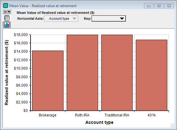
The main result of the model is Realized value at retirement. This represents the amount available for you to spend when you reach retirement, after taxes have been accounted for. Here is an example of the mean result, both table and graph view.
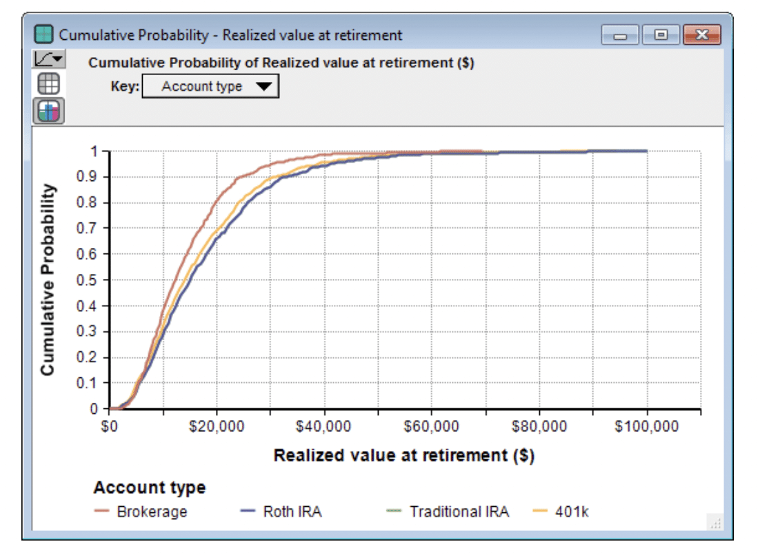
You can also look at the probability distribution of the result, here shown as a cumulative density (CDF)
From the CDF graph, you can read off that the probability of ending up with $20K or less from the initital $5K pre-tax investment is 80% for a brokerage account, but only 65% for a Roth IRA. The uncertainty modeled here is from the uncertainty is market performance.
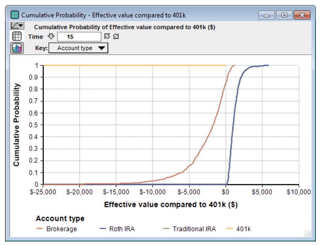
My objective with this model is to compare the relative performance of the different options, and not so much to the final value. Hence, I’ve included the Effective value compared to 401k result, with the CDF shown here
As predicted above in the section Income Tax, because I estimated my retirement income tax rate to be the same as my current income tax rate, the curves for Roth and traditional IRA are identical (the blue line in graph, exactly covering the green line). We can see that there is an 50% probability that these will outperform a 401(k) by $1000 or more (under the set of assumptions that I used). The sensitivity analysis, as well as the earlier mathematical analysis, reveals that this is attributable almost entirely to the larger annual maintenance fees in the 401(k) account. The red line shows that there is a 50% chance the 401(k) will outperform the brokerage account by $1,700 or more, with a 10% change it could be by more that $6,000.
Keep in mind that these all all based on one particular set of inputs. The results will be different for different assumptions about market return, tax rates, and trading behavior.
Investment total versus realized value
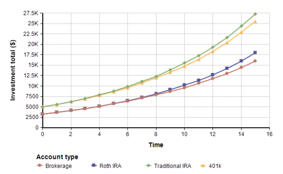
The model tracks the investment total as it simulates the returns over time, as seen here.
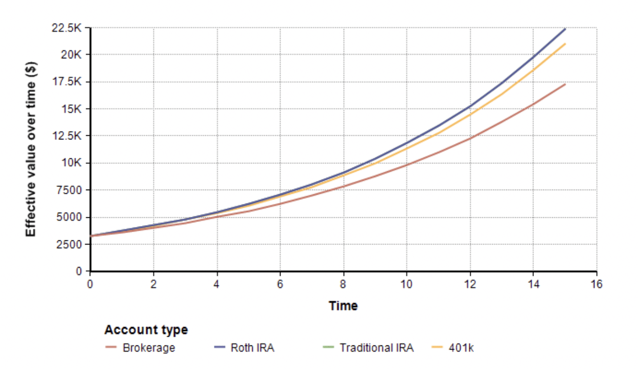
Although this is what you would see as your account balance as you track your account over time, it is misleading for comparison purposes because the taxes due in each case is different. I use the terms realized value, or effective value, to characterize the effective value to you at retirement, after subtracting off the taxes that will eventually come due. For the brokerage, I subtract off lingering capital gains that exist at the retirement boundary as if there were all long-term gains, whereas during the simulation the model estimates the likely mix of short-term versus long-term gains. Once this adjustment is made, the effective value of the above investment totals become
In this case, the effective value of a Roth and traditional IRA are identical, despite their investment value being quite different though the time horizon.
Sensitivity analysis
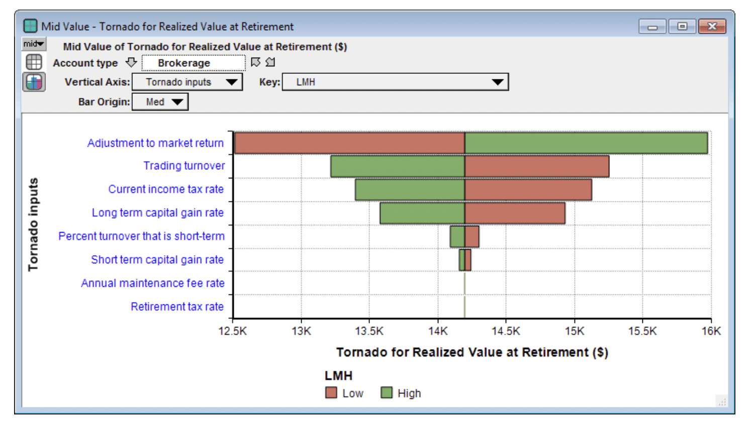
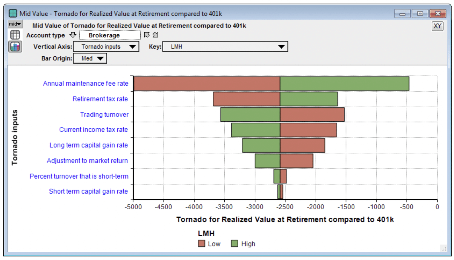
Once you have a quantitative model, you can use a sensitivity analysis to explore how much your conclusions depend on your particular inputs, assumptions, and estimates. Sometimes this understanding is more relevant to your decision making process than the numeric values of the computed results themselves. There are many different sensitivity analysis techniques and variations. What I’ve done here is explore what happens when you vary each input from a low to high value (where the original estimate, the base value, should be between the two). Once you’ve specified the high and low values, it is quite easy to create a Tornado Chart, such as the one shown here for the realized value at retirement for a brokerage account.
The most critical factor here to predicting eventual realized value is the Adjustment to market return. In this case, a 1% shift in either direction in the annual market return distribution impacts net performance more than other factors, with a change in trading turnover having the second largest effect (see the Compounding effect section above). On the other hand, when we look at the difference between the performance of a brokerage account compared to a 401(k) account,
now the relative performance is more sensitive to five other inputs that it is to a change in market performance (Adjustment to market return). What dominates the difference in performance between a brokerage and a 401k account, the annual maintenance fee of the 401k seems to be the most sensitive factor — i.e., a change in maintenance fee would have the largest impact on the relative performance.
In this model, I developed a new presentation of this sensitivity analysis in the form of an interactive sensitivity panel. The idea was from Max Henrion, who challenged me to use some of the new cell formatting features in Analytica 5, especially computed cell formats, in a MultiTable to merge information about the inputs (e.g., units), editable cells for low and high ranges, the input values themselves, also editable, then the computed sensitivity results in both number and bar form in the same cells, emanating from a centerline. The account type would be present as a slicer control. Some inputs would vary by account type (e.g., annual maintenance fees), while some would be the same across account types. The sensitivity panel for the realized value looks like this.

Summary
The main message here is that everyone’s situation is different, and the comparison between the different options depends on many inputs and assumptions that are probably different for you than they are for me. The tax advantages of 401(k)s or IRAs are helpful in general, but to understand how much difference they make in your case, I invite you to play with this model, and to even take it further and modify it and adapt it to explore other related issues.

