A shapefile (*.shp) is a binary file format used by Geographic Information Systems (GIS). I used an existing Python library (Fiona) to read and parse a shape file, and then imported that data into Analytica. Here I’ll show how I did it. This builds on last week’s blog article, How to call a Python function from Analytica with a more complex example. Kim Mullins at Lumina already made use of this to read in shapefiles of Gas Pipeline locations provided to us by PG&E for a project that Lumina is working on with them, and she’s used that to overlay the pipes on maps in the Analytica Cloud Platform. In this article, I’m using shape data for US states and territories in Analytica.
On the Python side, I made use of the same Analytica_Python.py library (module) from last week, as well as the Fiona module, to create the ShapeFileReader class shown here.
# -*- coding: utf-8 -*-
"""
Created on Thu Aug  2 07:28:31 2018

@author: Lonnie Chrisman, Lumina Decision Systems
"""

import Analytica_Python
import fiona

def flattenLists(l,sep):
    if isinstance(l,list):
        r = []
        for li in l:
            z = flattenLists(li,sep)
            if isinstance(z,list) and len(r)>0:
                r = r + [sep]
            if isinstance(z,list):
                r = r + z
            else:
                r = r + [z]
        return r
    else:
        return l

class ShapeFileReader :
    _reg_clsid_ = "{328E85D2-C8A9-4A9C-AD8C-8B61B78F2A56}"
    _reg_desc_ = "COM component that reads a shape for a .shp shape file"
    _reg_progid_ = "Lumina.ShapeFileReader"
    _reg_class_spec_ = "ShapeFileCOM.ShapeFileReader"
    _public_methods_ = ['open','numShapes','getShape','getProperty']
    _public_attrs_ = ['softspace', 'noCalls']
    _readonly_attrs_ = ['noCalls']

    def __init__(self):
        print("New " + self.__class__.__name__)
        self.softspace = 1
        self.noCalls = 0

    def open(self,filename):
        self.shapes = fiona.open(filename)
        return len(self.shapes)

    def numShapes(self):
        return len(self.shapes)

    def getShape(self,i):
        c = self.shapes[i-1]['geometry']['coordinates']
        return flattenLists(c,(None,None))

    def getProperty(self,i,prop):
        return self.shapes[i-1]['properties'][prop]


Analytica_Python.AddCOMClass(ShapeFileReader)

if __name__ == "__main__":
    Analytica_Python.TopLevelServer(__file__)
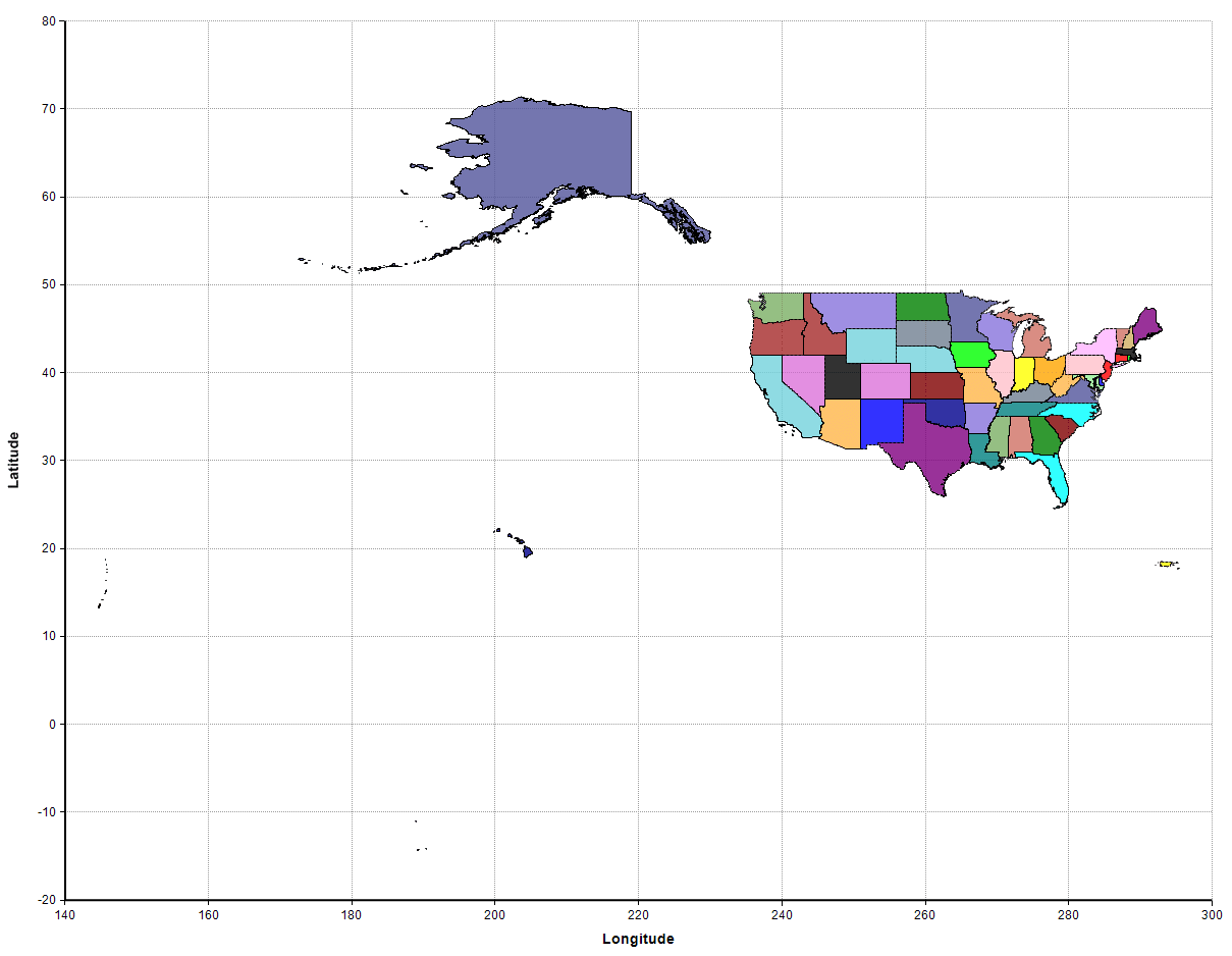
I used this to read the Cartographic Boundary Shapefiles of the 56 US states and territories from the US Census Bureau into Analytica, as plotted here from Analytica:
On the Analytica side. I instantiated the COM object and opened the file. Notice that the open() method of ShapeReader returns the number of shapes in the file.
Variable Shape_reader := COMCreateObject( "Lumina.ShapeFileReader" )
Variable Num_shapes := shape_reader->open(shape_file)
You can obtain the list of state and territory names using Shape_reader->getProperty(1..Num_shapes,'NAME'), but it isn’t in sorted order. To use the sorted names for an index, but also keep track of the original position, I computed both State and State_num from the same Definition:
Index State := ComputedBy( State_num )
Variable State_num :=LocalIndex unsorted := shape_reader->getProperty(1..Num_shapes,'NAME');
State := SortIndex(unsorted);
@[unsorted=State]
You can read the shape of California using Shape_reader->getShape(State_num[State='California']). The result has 2 indexes, the first index has a length of 5126 and indexs the points, the second has a length of 2 for the longitude and latitude. Similarly, you can read the shape of Michigan using Shape_reader->getShape(State_num[State='Michigan']). In this case, the first index has a length of 13,850 points. To make it easier to plot and manipulate the data in Analytica, I reindexes these onto the same two indexes. My Shape_segment index indexes the points, and has to be long enough for the longest shape (which happens to be Alaska, with 117,300 points). Hence, I defined my indexes as follows.
Variable Points_per_state :=for i:=State_num do IndexLength((shape_reader->getShape(i)).dim1)
Index Shape_segment := 1..Max(Points_per_state, State)
Index LatLong := ['Longitude','Latitude']
With these indexes, I read in each state and re-indexed it only these two indexes, so that I ended up with a 3-D array of shapes, indexed by State, Shape_segment and LatLong.
Variable State_shapes_orig :=Local si[]:=State_num do shape_reader->getShape(si)[@.dim1=Shape_segment,@.dim2=@LatLong]
When I first graphed this, Guam, the Mariannas, and several Aleutian islands appeared way over to the right.
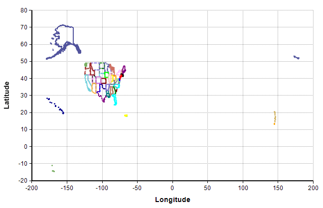
This happens because the shape file uses longitude numbers between -180 and 180 degrees. I adjusted those to be between 0 and 360 (in fact, between 140 and 300) for a more natural plot.
Variable State_shapes := If LatLong='Longitude' Then Mod(State_shapes_orig,360,pos:true) Else State_shapes_orig
That result is the first graph above, using a polygon fill.
This accomplished my first goal of extracting the data from the shapefile, but with 13 million points, it was too unwieldy for what I wanted it for. The shapes had far more resolution that I needed, with minute variations along coastlines, etc. I then continued from there to downsample, eliminating variations of less than 2km, except in the case of Alaska, where I eliminated variations of less than 20km. That turned out to be pretty challenging, and not within the scope of the current article, but the exercise reduced all state outlines to 3,163 points or less, which worked quite nicely for my purposes. I have further extracted that data into a stand-alone model (not requiring Python nor any advanced edition of Analytica) for those of you who would like to use these shapes for your own plots, such as this one:
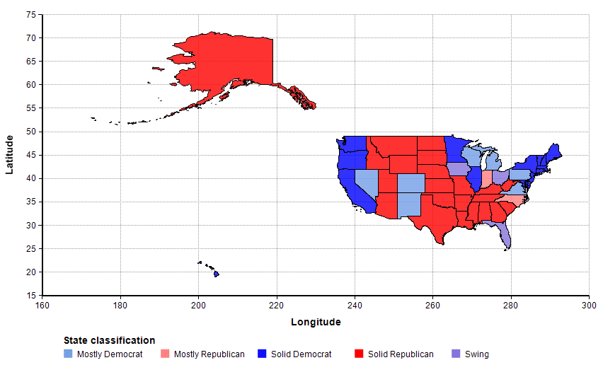
You can download the Red or blue state model if interested. It works with any edition of Analytica.
In summary, this blog extended the initial How to call a Python function from Analytica article with a more sophisticated example that parses and imports shapefile data into Analytica models.