Abstract: This article explores the difficult problem of estimating the mutual information between two variables from a sample of data. I use examples to demonstrate the challenges, and introduce a new algorithm for estimating mutual information along with an explicit representation of its uncertainty.
A measure of association is a function that rates the strength of statistical dependence between two variables. In casual talk, people often express this idea by asserting that two things are “correlated”; however, in statistics the term correlated has a more precise meaning, where correlation (or more precisely, Pearson correlation) is a measure of how linear a statistical dependence is. Also in common usage is rank correlation, which measures how monotonic a statistical dependency is. But many dependencies can elude these measures, motivating the use of other measures of association.
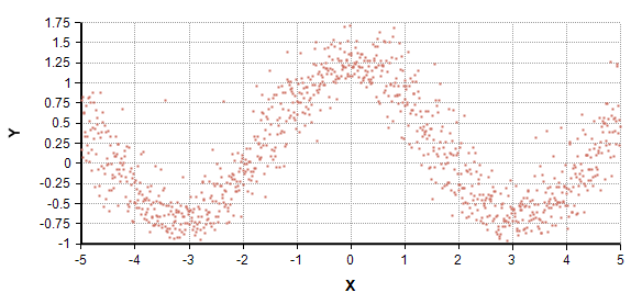 Figure 1: X & Y have a clear dependence, but correlation and rank correlation are zero.
Another possible measure is mutual information, I(x,y). In Figure 1, the variables have a zero correlation and zero rank correlation, but have 6.5 bits (4.5 nats) of mutual information (when x & y are each quantized into 32,000 distinct discrete values), demonstrating that this measure can pick up on dependencies undetected by straight correlation.
Although promising as a measure of association, it is difficult to estimate I(x,y) from empirical data. I will explore these difficulties in the remainder of this article, and introduce a new algorithm for doing so.
Mutual information
I limit the scope of this article to discrete variables and discrete probability distributions. The issues here are also important to estimation in the case with continuous variables, since estimation techniques often partition continuous values into discrete bins (Marek & Tichavský (2009)).
Given a joint probability distribution, P(x,y), over two discrete variables, the mutual information I(x,y) between x and y is defined as
$latex I(x,y) = sum_{x,y} P(x,y) ln {{P(x,y)}over{P(x) P(y)}}$
The sum excludes terms with $latex P(x,y)=0$. The base 2 logarithm is often used, in which case result is in units of bits. The natural logarithm can alternatively be used, in which case the result is in units of nats. In this article I use the natural log. The most important thing to notice about this definition is that it defines mutual information in terms of the underlying probability distribution, which is unknown to us when we are trying to estimate $latex I(x,y)$ from sample data.
Mutual information is always non-negative. It is zero when x and y are statistically independent. It is not limited to the range from 0 and 1, but it is always less than the entropy of each variable. The entropy of a variable is the mutual information of that variable with itself, $latex I(x,x)$.
$latex H(x) = I(x,x)$
$latex 0 le I(x,y) le minleft( H(x), H(y) right)$
Simple estimator
Let $latex (X_i, Y_i)$ be a data set of $latex N$ data points. To compute the empirical mutual information, count the frequencies of each combination of values, $latex freq(x,y)$, and then compute:
$latex freq(x) = sum_y freq(x,y)$
$latex freq(y) = sum_x freq(x,y)$
$latex I_N(x,y) = sum_{x,y} freq(x,y) ln {{freq(x,y)}over{freq(x) freq(y)}}$
when computing the sum, only terms where freq(x,y)>0.
Estimation bias
The simple estimator, $latex I_N(x,y)$, does not yield an unbiased estimate of $latex I(x,y)$. To illustrate this, I ran 1000 experiments. In each, I used Analytica to generate a randomized underlying joint probability distribution, from which I computed the underlying “true” mutual information, $latex I(x,y)$. Each of the two variables had 10 possible values. Using that distribution, I then sampled 100 data points and computed $latex I_N(x,y)$ via the simple estimator. The following plot compares the true underlying mutual information with the empirical $latex I_N(x,y)$ from the simple estimator.
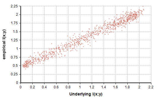
Each data point in the above graph corresponds to one experiment, there are 1000 points shown. Notice that when the true underlying $latex I(x,y)$ is 0.1, the simple estimator consistently returns a value around 0.6. These very poor estimates illustrate the inherent bias in the simple estimator. Figure 3 shows the difference between the estimated and actual, or sampling error.
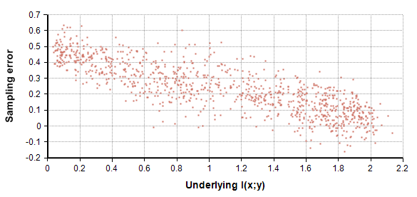
Figure 3 illustrates that the bias in the estimation decreases as the level of statistical dependence increases.
Independent variables
It is fairly easy to analyze the case of statistically independent variables. When x and y are independent, their mutual information is 0. But since the simple estimator only adds together positive quantities, it always returns a positive value, never reaching zero.
The simple estimation formula for the independent case, multiplied by $latex 2 N$, is the same as the G statistic used in a statistical G-test, and this statistic is known to have a chi-squared distribution (Harremoës & Tusnády (2012)).
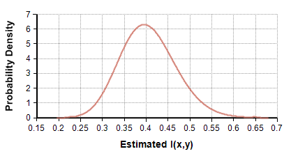
In Analytica, you can plot of the distribution for $latex I_N(x,y)$ using the expression
ChiSquared( (K-1)^2 ) / (2 * N)
where K are the number of distinct discrete values for x and for y, with K=10 in my example. N is the sample size and is 100. The plot shows that when x and y are independent, you can expect to get an estimated value around 0.4, and it is very unlikely you’ll see an estimate below 0.2.
The mean of this distribution, which is the mean bias of the simple estimator in the independent case, is $latex (K-1)^2/(2 N)$, the standard deviation is $latex (K-1)/(sqrt{2} N)$, which is 0.064 in the current example.
I experimented with independent variables, varying same sizes (N) and number of discrete outcomes (K), and found the theoretical distribution in Figure 4 is a perfect match to empirical simulations.
Dependent variables
In Figure 3, the dispersion of $latex I_N(x,y)$ is nearly twice the standard deviation predicted for the independent case. Plus, the bias in the estimate decreases as the underlying mutual information increases.
First, I obtain a mean estimate of the bias as follows. Empirically from Figure 3, we see that the mean bias decreases linearly as I(x,y) goes from the independent case to the maximum value, which I estimate as $latex min( H(x), H(y) )$. At I(x,y), the mean bias is $latex (K-1)^2 / (2 N)$, and at the maximum I(x,y) it is 0. From the data alone, we don’t have access to the true underlying I(x,y) or entropies H(x) and H(y), so we have to use $latex I_N(x,y)$ and $latex H_N = min( I_N(x,x), I_N(y,y) )$.
$latex E[ I_N(x,y) ] approx {( H_N – I_N(x,y) )over{H-c}} c$
where $latex c = (K-1)^2 / (2 N)$. This is an empirically derived formula for the E[ IN(x,y) ], not a mathematically derived one. I discovered through experimentation that a slightly improved fit results when you multiply $latex H_N$ by 0.8 before inserting it into the formula for E[ IN(x,y) ] — this twiddle reflects the reality that the empirical entropy is not a perfect estimator of the upper bound. With these adjustments, Figure 5 depicts the remaining sampling error.
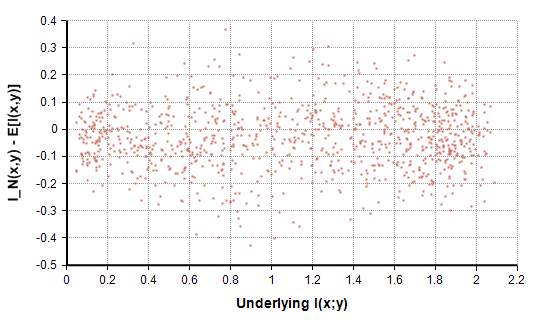
The thing to notice from Figure 5 is that the adjusted sampling error (the vertical axis) is centered around zero, demonstrating that the adjustment accounts correctly for the sampling bias across all levels of statistical dependence.
The standard deviation of the adjusted sampling error in Figure 5 is 0.12, compared to 0.064 when I(x,y)=0. This difference between the dispersion in the dependent and independent cases grows when we look at larger sample sizes. When the sample size is 1000, the empirical dispersion for the dependent case is about 5 times greater than for the independent case, and at N=10,000 it is 16 times greater. So the dispersion in sampling error evidently scales differently in the dependent and independent cases. The log-log plot it Figure 6 shows how increasing the sample size, N, decreases the empirical standard deviation for both the dependent and independent cases.
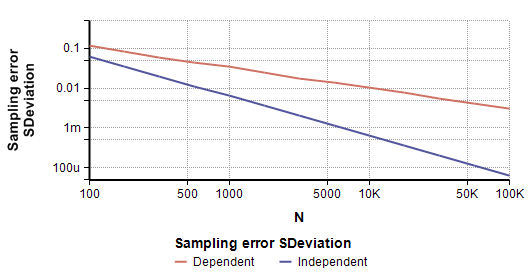
Figure 6 shows that the standard deviation in sampling error decreases linearly when plotted on a log-log plot for both the dependent and the independent cases, but whereas the slope is -1 for the independent case, it is -0.5 for the dependent case. This leads to the following formula for predicting the standard deviation is sampling error in $latex I_N(x,y)$ for dependent variables:
$latex sigma = gamma (K-1) / sqrt{2 N}$
Where $latex gamma=0.18$ accounts for the y-intercept in the log-log plot. Once again, this is an empirical observation, not a theorem.
Bias compensation
Numerous authors have advocated methods of subtracting the expected bias from the simple estimator as a way of obtaining an unbiased estimator of $latex I(x,y)$ (Miller (1955), Chee-Orts & Optican (1993), Hertz et al. (1992), Panzeri & Treves (1996)). To a crude first order, one can simply subtract $latex (K-1)^2/(2*N)$, the bias for the independent case. The various authors have approached this by finding various ways to obtain a more refined estimate of bias.
Bias subtraction has the obvious drawback that your estimation of I(x,y) after subtracting bias may be negative, which has no obvious interpretation. These papers generally focus on obtaining a single unbiased estimate of I(x,y), whereas I have an interest in obtaining information about the degree of uncertainty in the estimate (the Chee-Orts & Opticon (1993) method has potential to be adapted to include uncertainty). Several of the proposed bias compensation offsets depend only or the granularity of the discetization and the sample size, and therefore do not capture the effect depicted in Figure 3, where it is seen that the bias decreases with increasing statistical dependence. The algorithm that I introduce in the next section is intended to address these issues.
Estimation algorithm
In this section, I introduce a new algorithm for estimating the posterior distribution of I(x,y) from sampled data. I derive the algorithm by inverting sampling error of IN from the preceding sections. It is equivalent to using Bayes’ rule with a uniform prior over I(x,y).
The idea is depicted graphically as follows. Suppose we receive a data set and compute $latex I_N(x,y) = 1.1$. The empirical model derived in the preceding sections gives us a statistical model of the sampling error, which characterizing the scatter of the points in Figure 7. We take a slice at the measured value for $latex I_N(x,y)$ as shown by the dotted blue line.
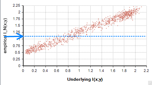
The posterior estimation of I(x,y) is a unimodal distribution along the blue dotted line in Figure 7. To make it easy to invert, I use the characterization of the bias to draw a line through the middle of the cloud of point, along with a band on each side. To do this, let
$latex y(x) = c + (1-c/{H_N}) x$
$latex c = (K-1)^2 / (2 N)$
$latex sigma = 0.18 (K-1) / sqrt{2 N}$
Note: I have found that substituting $latex 0.8 H_N$ for $latex H_N$ works better, and have done so in the graphs and results here.
Figure 9 plots y(x) along with $latex y(x) pm sigma$, which is a graphical depiction of the distribution of IN(x,y) as a function of I(x,y).
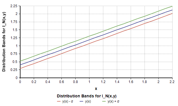
The bands depiction in Figure 8 is somewhat tailored to the actual data sample, unlike the scatter in Figure 7, since it used $latex H_N$. By inverting the lines in Figure 8, we obtain the posterior mean and standard deviation (ignoring the boundary at I(x,y)=0).
$latex mu_{post} = H_N ( I_N(x,y) – c) / (H_N – c)$
$latex sigma_{post} = sigma H_N / (H_N – c)$
We can then represent the posterior estimate of I(x,y) using a truncated Normal distribution. For example, in Analytica syntax,
Truncate( Normal( mu_post, sigma_post ), 0 )
Note that $latex mu_{post}$ and $latex sigma_{post}$ are not the final posterior mean and standard deviation — they are the mean and standard deviation of the Normal before Truncation.
Examples
All examples in this section use discrete variables having K=10 possible values.
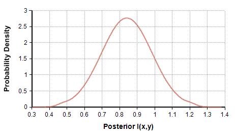
In the first example, I sampled N=100 points from a distribution having I(x,y)=0.736. The sample information was $latex I_N(x,y)=1.1$. The estimation algorithm produces posterior estimate shown in Figure 9.
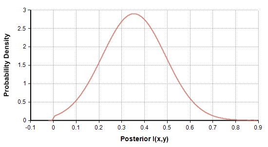
In the second example, I sampled N=100 points from a distribution having I(x,y)=0.33. The empirical $latex I_N(x,y)=0.7$ and the posterior is shown in Figure 10.
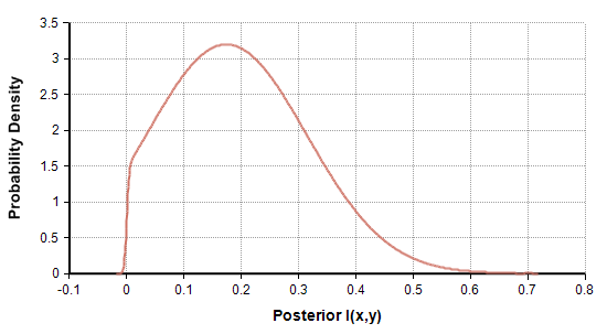
The third example sampled N=100 points from an underlying distribution having I(x,y)=0.046. The empirical information was 0.55 and the posterior estimate for I(x,y) is shown in Figure 11.
Summary
Mutual information can capture complex associations between variables that are missed by standard correlation measures. However, estimating the underlying mutual estimation from a data sample is challenging, due to an inherent bias present in the empirical mutual information. In left uncompensated, this bias magnifies the apparent degree of statistical dependence for cases having little or no dependence.
This article introduces a new Bayesian-style algorithm, derived from an empirical study across a sampling of distributions, for estimating I(x,y) from a data sample, with an explicit representation of the uncertainty in the estimate.
You may find it disturbing that I developed the algorithm from an empirical study. It is entirely possible that my sampling of underlying distributions is not representative of a distribution you encounter in your own application, and that could throw off the quality of the results. If you are academically minded, you may find the absence of an analytical derivation behind the algorithm to be disconcerting. These are all valid criticisms.
References
- M. N. Chee-Orts & L. M. Opticon (1993), Cluster method for the analysis of transmitted information in multivariate neuronal data. Biol. Cybernetics 69:29-35.
- P. Harremoës & G. Tusnády (2012), Information divergence is more Χ^2-distributed than the Χ^2-statistics.
- J. A. Hertz, T. W. Kjaer, E. N. Eskander and B. J. Richmond (1992), Measuring natural neural processing with artificial neural networks. Int. J. Neural Systems 3 supplement 91-103.
- T. Marek & P. Tichavský (2009), On the estimation of mutual information, ROBUST 2008, JCMF 2009:263-269.
- G. A. Miller (1955), Note on the bias on information estimates. Information Theory in Psychology: Problems and Methods II-B:95-100.
- S. Panzeri & A. Treves (1996), Analytical estimates of limited sampling biases in different information measures. Network Computation in Neural Systems 7:87-107.


